Carbon Pricing Isn’t Effective at Reducing CO2 Emissions

How does carbon pricing affect macroeconomic balance and ultimately CO2 emission? What about electric vehicles that are now being promoted by the Biden administration?

Economists’ standard advice for controlling global warming is to impose a high price on emitting CO2, which is said to discourage carbon-intensive activities and induce carbon-saving technical change. In a recent review of the New Deal, William Janeway (2021) draws a distinction between efficient and effective policies. He comes close to economist-speak by describing efficiency as a low-cost means for moving toward a desired goal. Whether an efficient intervention will be effective in reaching the goal is another question altogether. In the short- to medium-run, raising carbon prices within a politically acceptable range may be efficient at inducing macroeconomically small changes in the structure of the economy and level of emission. But the move will not be effective, because the changes will remain small for at least three reasons.

Energy constitutes a relatively small proportion of economic activity. It is crucial for the functioning of the macro system, but usually is not the tail that wags the dog.

Carbon pricing brings in the “little triangles” of economic welfare analysis applied by Arnold Harberger (1954, 1971), which are not significant in terms of GDP (James Tobin, 1977). The reason, as illustrated below, is that the percentage change in, say, gasoline demand in response to a higher tax is the product of a negative price elasticity of demand which is a fraction of the percentage change in price, typically less than 100%. The product of two fractions is smaller than both, meaning that the demand response is weak. Even if the magnitude of the long-run elasticity is bigger than the short-run value (say -0.4 < -0.2 or 0.4 > 0.2), the conclusion remains.

Finally, following Harberger and lurching into jargon, economists usually assume that the proceeds of a tax are passed in “lump sum” fashion back to consumers. This transfer produces an “income effect” stimulating demand for all goods including gasoline. The increase can partially offset the price-induced demand reduction due to “substitution” of other goods for lower purchases of gasoline. Substitution effects almost always dominate income effects, so that most of the transferred income gets spent on non-energy goods and services. Total gasoline consumption still declines.

Somewhat similar reasoning applies to electric vehicles (EVs). They have a great advantage in delivering around 70% of the energy they use for moving the vehicle as opposed to 25% for internal combustion engine (ICE) counterparts. But the electricity has to come from some source. As of now 60% of the energy going toward electricity generation in the USA comes from fossil fuels. Unless that share is substantially reduced, EVs will not shift energy accounting by very much. They are efficient in reducing end-use of petroleum in the transport sector, but not effective in controlling CO2. Details appear below.

Energy and economic accounting in a SAM

To make the arguments as clearly as possible, the paper sets out an economy-wide social accounting matrix (SAM) combining energy and national income in one place. An introductory one-sector SAM in Table 1 is extended in Table 2 to a matrix with non-energy (90% of the economy) and energy sectors. Calculation shows how higher national carbon prices will have minimal short- to medium-term effects.

With its relatively low carbon prices, the USA is far behind the rest of the world in attacking global warming. A gallon of gasoline costs around $2.50 here vs. at least $7.00 in Western Europe. Reducing global warming from the American side would have to combine reductions or mitigation of CO2 emission with technical change to cut back the two-thirds share of primary energy not put to economically productive ends. Higher carbon prices at most could be a necessary but not sufficient condition for such changes to occur. Details are sketched below.

The SAM in Table 1 introduces the numbers. The accounting conventions are that entries in the rows of the matrix are valued at the same price and that sums of entries in corresponding rows and columns (say sources and uses of household income) should be equal.

Macroeconomic data come from the national income and product accounts (NIPA) of the US Bureau of Economic Analysis reporting economic activity. Flows of energy use per unit time (so we are really talking about power) are lifted from charts generated by Livermore National Labs:

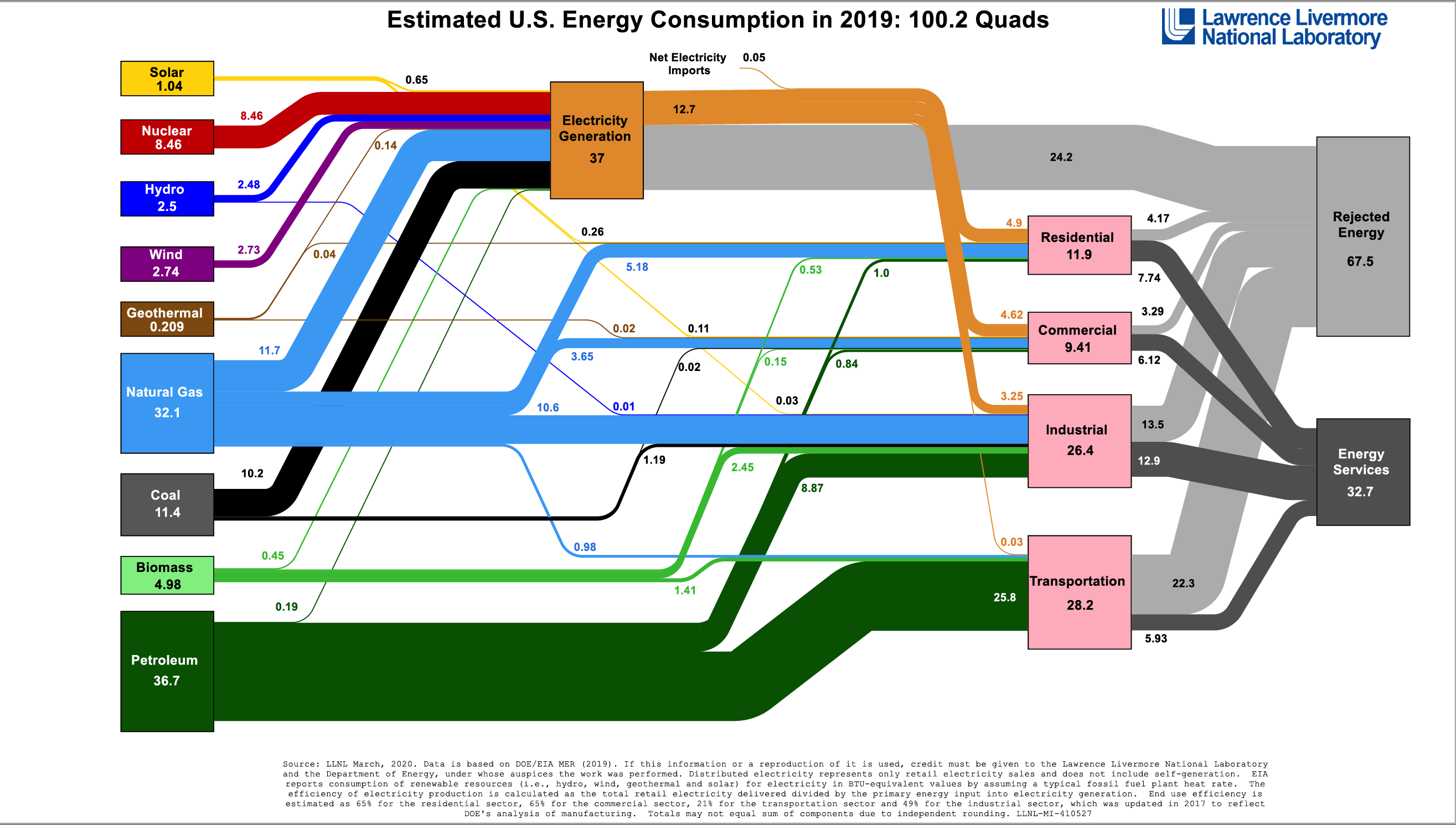
In both technical usage and popular discussion, energy flows and CO2 or carbon emissions per unit of time are quantified with a bewildering array of numbers. Livermore’s estimates are expressed in units of quadrillion British thermal units or quads of energy per year. US 2019 annual primary power use was 100.2 quads. In international standard (SI) units, the implied rate of power consumption was 3.38 terawatts, on the low side in comparison to other US estimates.

The SAM in Table 1 shows that the total value-added in 2019 was $21.4 trillion. Probably around 10% ($2 trillion) was supported by primary energy, mostly fossil fuels as shown in the Livermore diagram. One quad per year of primary energy roughly generates $20 billion of value-added (one terawatt supports $592 billion). Total US carbon (not CO2) emissions in 2019 were 1.39 billion tonnes.[1] GDP per unit of emissions was $15.4 million, and energy value-added per tonne was $1.54 million. The ratio of one billion tonnes of carbon emission in response to one trillion dollars of value-added was 0.065.

In Livermore’s usage, two-thirds of primary energy is “rejected” in line with the first and second laws of thermodynamics (“wasted” might be a better word). The energy put to use amounts to 32.7 quads or $754 billion of value-added. Residential and transport services, mostly used for consumption by households, absorb 13.7 quads or $274 billion. The remaining unwasted energy value-added of $480 billion is used for electricity generation, commercial services, and industry. The value of rejected energy is split between $800 billion from production and $500 billion from consumption.

The other entries in the SAM come from NIPA numbers – household and government consumption get separate columns, with exports and investment bundled together. The cost column includes the usual major flows. Adopting SAM accounting conventions, household income of $15.4 trillion comes from both wage and non-wage sources. It is used for consumption of $14.6 trillion and saving of $800 billion.

It seems clear that the Table 1 accounting should be expanded to include energy and non-energy sectors explicitly, with interindustry transactions built into the structure of costs. This extension will allow us to look in detail at how price changes impact the composition of consumption, value-added, and energy rejection. As noted above, adverse macroeconomic repercussions transmitted through the accounting will limit the effectiveness of carbon pricing in reducing the use of fossil fuel energy.

Table 1: SAM with values of energy flows 2019 (trillions of dollars)

Two-sector SAM

Table 2 shows a SAM which includes non-energy and energy-producing sectors with intermediate input-output transactions between them. To a large extent, the numbers about to be described follow from accounting restrictions in the SAM. They are illustrative, but their imprecision is irrelevant to understanding key energy vs non-energy linkages. All economic activities are assumed to be equally energy-intensive, for a first-cut macro analysis.

Table 2: SAM with non-energy and energy flows 2019 (trillions of dollars)

For both sectors, all components of both output and final demand are scaled to value-added. This assumption helps determine the interindustry transactions shown toward the upper left. In the Livermore data, electricity generation uses 37 quads or $700 billion of primary energy to generate 12.7 quads of usable energy.[2] If intermediate non-energy to energy sales equal $100 billion, then the gross value of energy output (the sum of the cost entries in the relevant column) will be $3 trillion.

If households take up the bulk of residential and transport services, their consumption of energy value-added will be $300 billion. The implication of equal row and column sums of energy flows is that energy to non-energy intermediate sales must be $1 trillion, channeled via the Livermore estimate of 19 quads or $3.8 trillion of commercial and industrial energy services. All these energy numbers are small in comparison to non-energy flows although the implied energy-to-energy input-output coefficient of 0.8 / 3 = 0.27 is rather large.

On the non-energy side, if “own” within-sector intermediate sales are $100 billion, then demand for output becomes $23.5 trillion. The sum of costs is $23.4 trillion, close enough for present purposes.

Two large transfer flows also enter the accounting. One is from government to households, financed by taxes and borrowing. It will be important in analyzing the impacts of carbon pricing. Households get $3.1 trillion in non-wage transfer income from the government, more than ten percent of GDP. In turn, there are taxes on various income flows and fiscal negative saving (higher spending than income) of -1.6 trillion.

The other transfer flow involves net payments of interest and dividends from business, government, and the rest of the world (RoW) of $2.6 trillion to (mostly high income) households. Like fiscal transfers and energy flows these payments amount to ten percent of GDP and reflect the big role of finance in the American economy.[3]

Gasoline and energy taxes and transfers

Now consider the impact of a tax on consumption of energy services. A hypothetical tax on gasoline can add numerical perspective. One gallon contains 5.5 pounds or 2.5 kilograms of carbon, implying that 400 gallons contain one tonne. If gasoline costs two dollars per gallon, then a fifty percent tax of one dollar would raise $400 per tonne of carbon, at the high end of the range of prices now being discussed in the literature.

The implied change in energy use is

Energy consumption change = Price elasticity x 0.5 x Initial use.

Table 2 shows that final sales from the energy sector are $1.3 trillion, including $520 billion for gasoline. A high magnitude estimate of the short-run price elasticity would be -0.2 so that the fall in energy consumption would be $0.2 x 0.5 x 0.52 trillion = $0.052 trillion. A decrease of $52 billion in gasoline consumption is trivial in macroeconomic terms.[4] From the ratio of carbon emissions to value-added quoted above, the annual total of 1.39 billion tonnes would fall by 0.065 x 0.052 = 3.4 million tonnes. Reduced emissions would still be nugatory at 8 million tonnes even if the 26.5 quads ($0.05 trillion) of rejected energy associated with residential and transportation services is taken into account. A long-run price elasticity of -0.4 would not change these results substantially.

The usual recommendation is that the proceeds of an energy consumption tax should be passed back to consumers. If the amount is estimated as the new price times the change in consumption, it will be $1.5 x 0.03 trillion = $0.045 trillion. An overestimate of the rebate could be based on total household energy consumption. The amount would be $0.45 trillion or $450 billion. Either way, the transfer is small in comparison to the existing flow (Social Security, Medicare, Medicaid, etc.) of $3.1 trillion in the SAM. The rebate amounts to a shift of three percent of initial total consumption. If income elasticities of demand are both equal to one, energy consumption in response to the initial version of the transfer would rebound by around ten billion dollars (against the “substitution” response of $52 billion). Non-energy purchases would rise by $130 billion.

A Harberger triangle supposedly measures the change in economic welfare associated with a change in a tax or subsidy. In comparison to macroeconomic aggregates, estimates are almost always small along the lines just discussed. The price manipulation, however, affects the whole existing volume of sales. A five percent tax applied to $520 billion of gasoline purchases would bring in $26 billion. Republican grandees James Baker and George Schultz in connection with a Climate Leadership Council (2019) proposed a carbon tax of $40 per tonne of CO2 or $147 per tonne of carbon, with proceeds to be distributed as a “dividend” to US households. US 2019 volume gasoline sales were 146 billion gallons. The resulting tax and transfer would be $53 billion, which can be compared to total fiscal payments of $3.1 trillion mentioned above. Applying a similar tax to all final energy sales would provide $230 billion.

With 129 million households, the carbon dividend from a gasoline tax would provide each one with around $400. A similar tax on all energy sales would increase the transfer to $1800. We are still not talking about a big amount of money in comparison to GDP or even pre-existing fiscal transfer flows. Needless to say, “extraordinary” transfers associated with the COVID pandemic were much larger.

The bottom line is that a tax on household consumption of energy services would have very modest impact economy-wide. These results are fully in line with Harberger’s (1954) original paper, which argued that the effects of “distortions” due to monopoly are small. His little triangles carry over to considerations of energy use. Tobin’s (1977) old observation that “It takes a heap of Harberger triangles to fill an Okun gap” neatly summarizes the situation.

Similar conclusions apply to movements in input-output coefficients due to higher energy costs in production. That is, a tax on energy costs would presumably induce lower (higher) input-output coefficients for energy (non-energy) interindustry sales. With typical elasticities of substitution, the shifts would be small in macroeconomic terms.

Other alternatives, electric vehicles, and Biden

Within American political limitations on raising carbon prices (can you imagine even $5 per gallon for gasoline?), the standard economists’ recommendation for reducing global warming does not have traction. The key tasks are to cut into energy consumption by other means and to offset CO2 emission generated by a given level of power applied to economic ends. Economists lack the technical skills to deal seriously with either issue but a few observations make sense.

The Livermore diagram shows that of the 37 quads of energy flowing to electricity generation, 21.9 come from coal (10.2) and natural gas (11.7). Given the well-known difference in the rate of CO2 emission from the two fuels, replacement of coal by gas and much more importantly by non-fossil sources of energy makes sense.

Similarly, electricity in principle can replace a portion of the 26 quads ($520 billion, 2.5% of GDP) of petroleum used for transportation, of which 22 quads are rejected. President Biden’s energy proposals put emphasis on electric vehicles. Again we meet Janeway’s contrast between a relatively efficient policy initiative and one that is effective in reducing global warming.

A big network of charging stations and subsidies on purchases are important components of the package. But suppose that over the next few years, EVs replace two quads of the six that go from petroleum to transportation services, along with 7.3 quads of wasted energy. Of total carbon emission of 1.39 billion tonnes in 2019, the reduction that EVs might permit is 0.25 x 4.6 x 1.39 = 160 million tonnes. This is a significant number but less than 12% of total emissions. The result is the familiar consequence of multiplying two fractions. Big reductions in emission would have to come from replacing fossil fuel with renewable primary energy sources and/or carbon sequestration.

There are many such examples. In a book written for MIT undergraduates, Jaffe and Taylor (2018) lay out options at a somewhat technical level. Grubb et.al. (2014) do the same with less physics and chemistry.

Economists also have other theories. Stiglitz (2019) considers “induced innovation” over time in terms of trade-offs between increases in energy and labor productivity responding to shifts in the cost of carbon. Like most of the literature, the discussion is largely theoretical. Stiglitz conveniently ignores the fact that labor and energy productivity levels have increased at close to equal rates for centuries (Semieniuk et. al., 2021). He also examines the welfare impacts of carbon taxes and subsidies, treating them as macroeconomically crucial. The discussion above shows how they are in fact insignificant in the relevant range of magnitude.

As of this writing, the Biden infrastructure and energy plan appears to be in a state of flux. Carbon prices are not central, although stable, relatively high levels could support rates of energy productivity growth in line with labor productivity (the historical pattern). Along with supporting EVs, tighter regulation along with subsidies and new investment in the vicinity of the $200 billion per year are likely to figure. The practical task will be to make sure that these interventions produce tangible results. These are largely issues about specific technologies, not carbon pricing.

Even more fundamental, in the USA the government since WWII has pursued a policy of keeping energy prices low, which is one of the main long-term determinants of the urban sprawl and other characteristics of spatial-social organization now. Carbon pricing is part of this policy outcome, but may be more a symptom of deeper socioeconomic forces than a cause. Harberger triangles and Baker-Schultz carbon dividends just scratch the surface.

References

Climate Leadership Council (2019) “The Four Pillars of Our Carbon Dividends Plan,” https://clcouncil.org/our-plan…

Grubb, Michael, with Jean-Charles Hourlade and Kersten Neuhoff (2014) Planetary Economics, New York: Reuters.

Harberger, Arnold C.(1954) “Monopoly and Resource Allocation,” American Economic Review, 44:2: 77-87.

Harberger, Arnold C. (1971) “Three basic postulates for applied welfare analysis,” Journal of Economic Literature, 9: 785-797.

Jaffe, Robert L., and Washington Taylor, The Physics of Energy, New York: Cambridge University Press.

Janeway, William (2021) “Lessons from the First New Deal for the Next One,” https://www.ineteconomics.org/…

Semieniuk, Gregor, Lance Taylor, Armon Rezai, and Duncan Foley (2021) “Plausible energy demand patterns in a growing global economy with climate policy,” Nature Climate Change, 11: 313–318.

Stiglitz, Joseph E. (2019) “Addressing climate change through price and non-price interventions,” European Economic Review, 119: 594-612.

Tobin, James (1977) “How Dead is Keynes?” Economic Inquiry, 15: 459-468.

Notes

[1] A metric “tonne” weighs 2205 pounds. To get to tonnes of CO2 emission as usually discussed by politicians and public, multiply the number for pure carbon by 3.67 or eleven thirds.

[2] The implied generation efficiency of 34% is close to thermodynamic limits.

[3] Share buybacks of a trillion per year could be included but are basically portfolio shifts between households and business and do not fit into standard national accounting.

[4] A useful rule of thumb is that a macro perturbation of less than one percent of GDP is irrelevant for practical purposes.

Acknowledgments

Support from the Institute for New Economic Thinking and comments from Thomas Ferguson, Nelson Barbosa, and Duncan Foley are gratefully acknowledged.