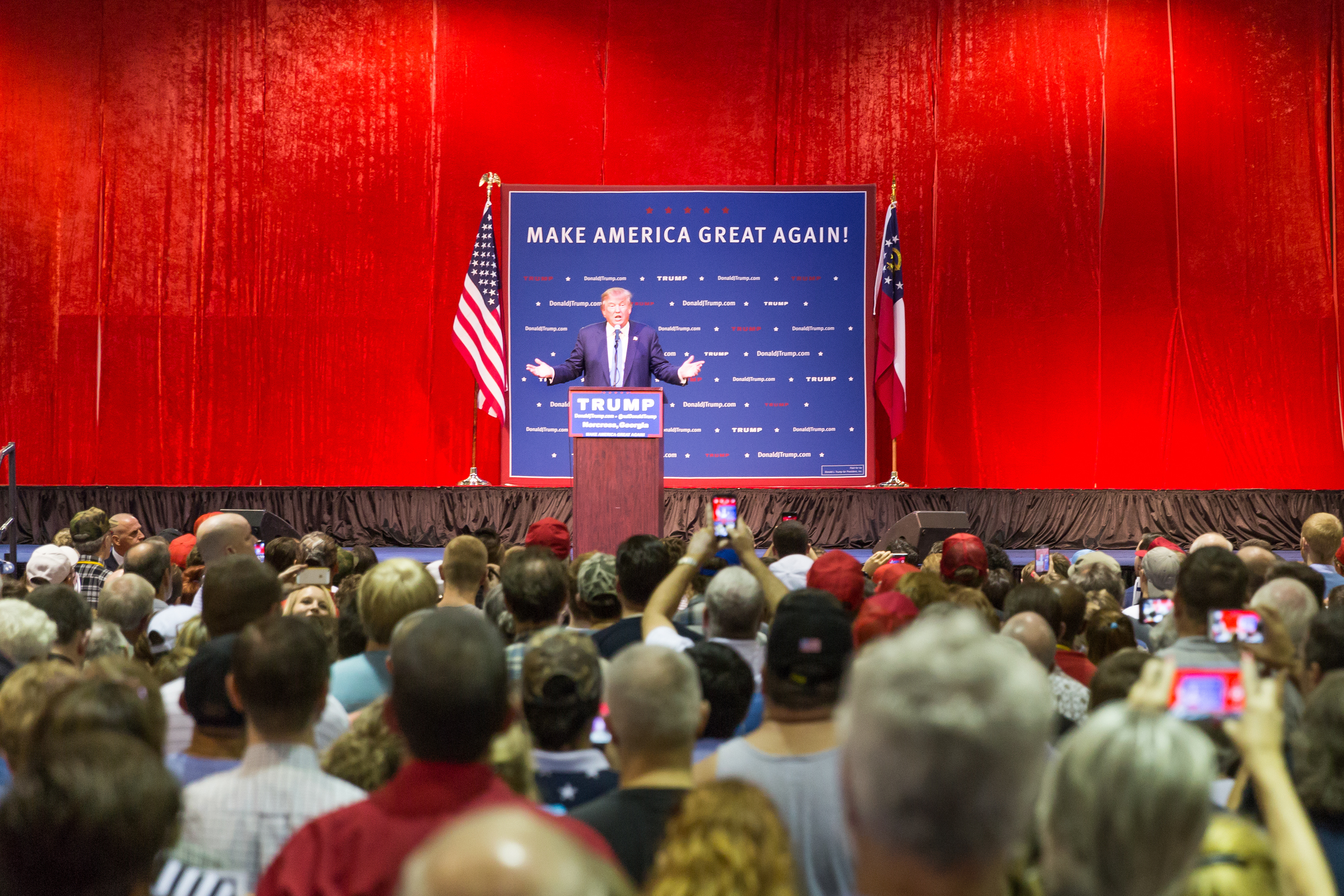
Economic issues are a primary part of Trump’s appeal to his base
A new note from the editors (2/15/2024):
INET recently published an analysis of the Republican vote in the 2024 New Hampshire primary that revealed a pattern of support for Donald Trump eerily similar to the vote for Senator Bernie Sanders in the 2020 Democratic primary: towns with lower median incomes tilted more heavily for the former President, just as they had in favor of Sanders against Clinton. In 2024, long-term town growth patterns accentuated this effect: slower-growing towns supported Trump at higher rates and affected the strength of income’s impact on the balloting. Put simply: lower incomes and slower growth over time interacted to raise Trump’s vote.
Since then Trump has weighed in dramatically on deliberations among Congressional Republicans over aid to Ukraine, the border, and other issues.
From the start INET emphasized the importance of understanding Trump’s appeal not simply in cultural terms – in plain English, all the dog whistles summoning racial, gender, and other stereotypes – but also economic issues. With the American government grinding to a halt over vital issues, it seems timely to repost an earlier INET study by Thomas Ferguson, Paul Jorgensen, and Jie Chen. This used machine learning techniques to compare support for Trump with that for Republican congressional candidates. In contrast to most published studies using machine learning, the paper deliberately compared the results of several leading algorithms. The factors that all three methods converged upon run very much in the grain of the New Hampshire results.
As incitements to genuine fear and trembling, credible invocations of the end of the world are hard to top. So when President Joe Biden mentioned the war in Ukraine and Armageddon in the same breath at a Democratic Party fundraiser, the whole world jumped. Amid a wave of news clips filled with swooning commentary and verbal handwringing, the White House staff rushed to do damage control.1
Yet scary as it was – and is, because what the President discussed is all too real – it is possible to doubt whether allusions to Armageddon fully capture the precarious state of the world today. After all, the classic vision of the Apocalypse in the Book of Revelations starred only Four Horsemen: Pestilence, War, Famine, and Death. The Fearsome Four are all obviously romping over the globe and not just in Ukraine. But nowadays the quartet travels in the company of a veritable thundering herd of other monsters: creatures representing serial climate disaster, inflation, rising interest rates, looming global debt crisis, and broken supply chains, to reel off a few. Not the least of the newcomers is one native to the USA: the prospect that the U.S. midterm elections may confer significant power on a true anti-system party akin to those that terminated the Weimar Republic.
A real understanding of this latest sign of the End Times requires something that even the exceptionally venturesome special House panel investigating January 6th has yet to produce: a detailed analysis of the plotters’ financing and links to the byzantine web of big money that sustains different factions within the Republican Party. (We are very far from considering the GOP as a unitary organism, even if the functional importance of the cleavages is an open question.)
But with the financing of January 6th still shrouded in Stygian darkness, we think a fresh analysis of the voting base of the Trump wing of the Republican Party provides a perfect opportunity to test out twenty-first century machine learning techniques to see if they might shed additional light on the roots of Trump’s appeal. Could they perhaps yield new evidence on the hotly disputed question of how much economic issues matter to Trump voters?
With polls showing that inflation tops the concerns of many voters across virtually all demographic groups, this is perhaps an odd question to pick up on now. But in the last few weeks, many pundits have noticed the relative absence of economic issues in Democratic messaging.2 The party has been emphasizing abortion and Roe vs. Wade. Many academic and literary commentators also continue to short the importance of economic issues in rallying support for Trump, even if we think the evidence is now overwhelming that his secret sauce was precisely a mix of racial and gender appeals with very clear economic ones. As a recent piece in the New York Times analyzing Trump voters illustrates, mainstream pundits still treat the subject like cats playing with balls of yarn: they do everything except digest them.3
The research we report here says nothing directly about 2022. But its findings are highly relevant to the election and, we suspect, what comes afterward, even if Congressional elections typically differ drastically from those in which the White House is in play.4 Our idea is straightforward: We search out the factors that drove the Trump vote in counties where he ran ahead of serious Republican congressional contenders in 2020. This is certainly only one of several plausible approaches to sizing up the former President’s leverage within the party, but we think it is more reliable than, for example, tracking districts in which 2022 candidates maintain the pretense that the election was stolen – that tactic likely pays with almost any size contingent of Trump enthusiasts.5
Selecting the most appropriate districts for this exercise requires some care, since we want to exclude ballot artefacts. We eliminated districts in which Republican House candidates obtained 100% of all votes cast. Our reasoning is that if no one, even a minority party candidate, showed on the ballot, the result, to put it politely, may not have reflected an affirmative choice for the House candidate in preference to the President. As long as some minor party candidates qualified for the ballot, though, we counted districts in the sample, even if no Democrat was on the ballot. We had analogous concerns at the other end of the scales. Where no or merely ceremonial Republican congressional candidates ran, the President’s margins over the sacrificial lambs could be equally artificial. We want to exclude both sets of cases, since they likely distort the relative attractions of Trump and Republican House candidates to the President’s mass base. The token cases also probably have little bearing on Trump’s leverage with Congressional Republicans, an issue which, no matter how the 2022 elections come out, is likely to be of burning future interest. We thus exclude races in which Republican congressional candidates failed to attain at least 35% of the vote. We readily acknowledge that no system of controls is perfect and that because county votes can be split up among several congressional districts either honestly or, more likely, due to gerrymandering, it is impossible to eliminate “organizational” artefacts altogether. Figure 1 shows a map displaying how district margins varied across the United States under our criteria.
Figure 1
Difference Trump Vote From Republican House Candidates in Sample
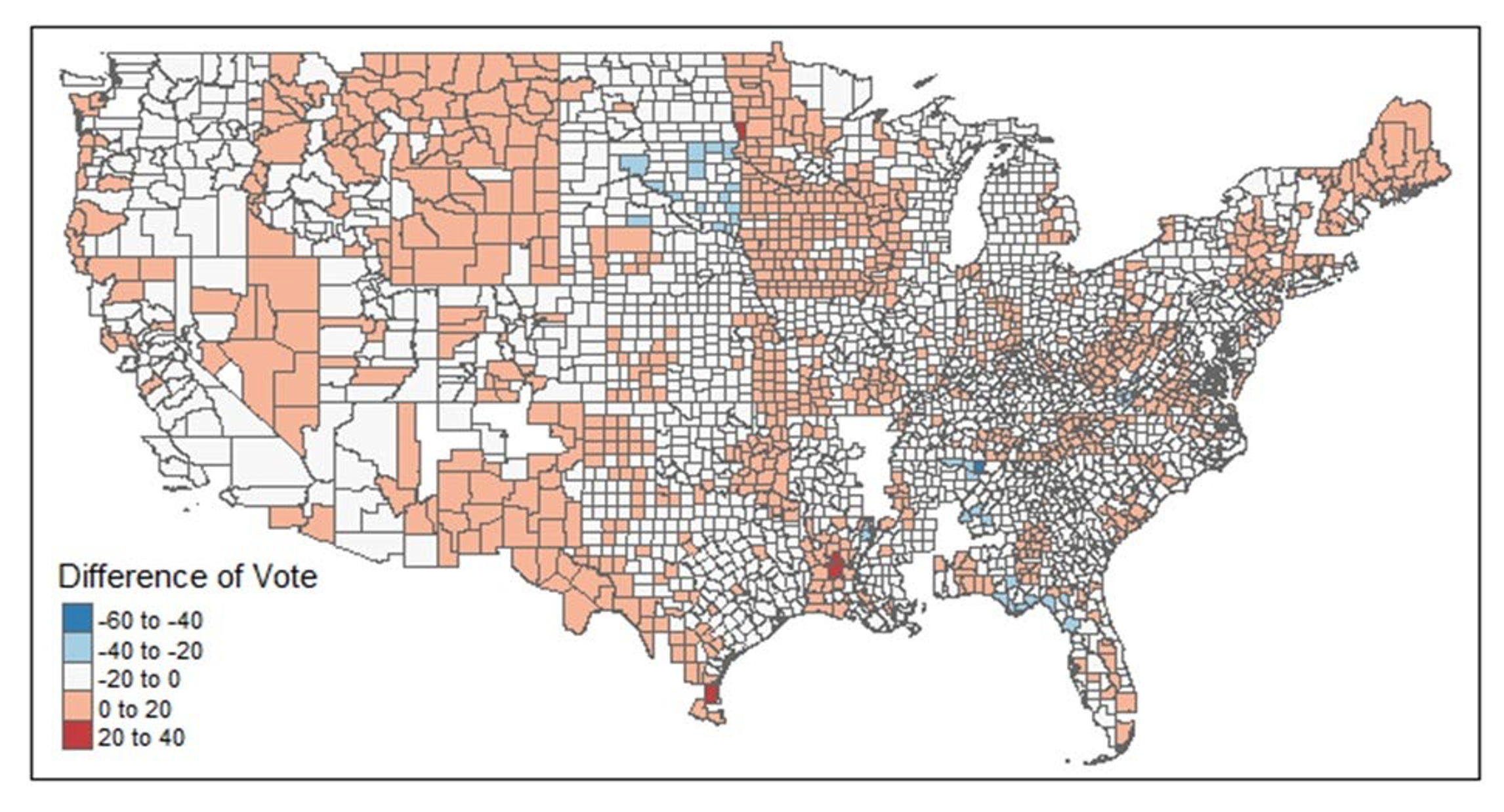
Source: Data From Ferguson, Jorgensen, and Chen, 2021; See Text on exclusions, etc.
This paper builds heavily off our earlier analysis of the 2020 election.6 Like that discussion, it relies not on national poll data, but county-level election returns. That approach has both advantages and disadvantages. The towering advantage is that the importance of place is intrinsic to the method. This permits studies of questions that are difficult or impossible drawing only on data from nationally representative samples of voters or normal exit polls. Those typically have too few cases in any one locality to sort out anything important. Many surveys, indeed, deliberately mask crucial details such as the towns in which voters live to preserve confidentiality.
Especially where Trump is concerned, studies rooted in national polls thus failed to catch many revealing facts. One we often point to is the finding – since paralleled in studies of “populist” movements in other countries — that in 2016 voters who lived in congressional districts with poorly maintained bridges disproportionately favored Trump, holding other factors, including income, constant.7 Or our results for 2020 indicating that in contrast with 2016, counties along the Mexican border voted in favor of the President more heavily than others as did counties with high percentages of Mormons. Perhaps the most striking result of all, however, was the evidence that study produced of the gigantic political business cycle that the Trump team engineered for certain crops in agriculture in its vain effort to win a second term. Such a result – which puts an entirely different face on the celebrated question of how Trump amassed so many votes in 2020 – is virtually impossible to discover unless one looks for it by searching out influences of specific industrial structures on voters (not simply campaign contributions – the focus of much of our other work).8
But a focus on aggregate, place-based voting returns also comes with costs. These need to be acknowledged up front. Some important questions become difficult or impossible to address. Our earlier paper spells out the drawbacks in detail, so our discussion here will be brief. The key point is that all of our findings concern patterns of aggregate data. There is a vast literature on the so-called “ecological fallacy” in statistics warning about what can go wrong in reasoning from wholes to parts in the behavior of particular individuals:
The way patterns at aggregate levels translate into the behavior of individuals is often far more complicated than readily imagined. Often what appears to be a straightforward inference from general results to specific voters is deceptive. Before surveys became ubiquitous, for example, election analysts often drew their evidence about how specific ethnic groups voted from returns in precincts where the group lived en masse. That skipped past questions about whether voters in less concentrated areas might be different or whether other groups in the district might alter their behavior in response and change overall results.9
The corollary is that certain issues of great interest, including how individuals combine issues of race, gender, and the economy in their individual voting decisions are not well approached through aggregate approaches. For that one wants observations on individuals, too, and our earlier paper waved yellow caution flags at many points.10
This paper requires even more forewarnings because it employs a form of machine learning, so-called random forest techniques. The potential pitfalls are numerous and require mention.
First comes a very general issue. Machine learning as a field has developed rapidly, mostly outside the boundaries of traditional statistics. It thrives in computer science departments, giant corporations, companies hoping to be acquired by those, and technically oriented government agencies and labs. Many of its products have a well-deserved reputation for being opaque. The field’s best-known methods – random forests, neural networks, and programs for parsing texts and natural language – are now diffusing rapidly into parts of the natural sciences and medicine, especially genetics, but their use across the social sciences is less common.11 The reception of both random forests and neural networks within economics and political science has been, we think, exceptionally cool. This despite widely trumpeted claims by some economists that resort to “big data” will somehow suffice to solve many traditional problems of economics.
The issues at stake in these debates are too big for this essay to treat in any depth. We will simply state our view that researchers have good reasons to be wary of machine learning. We have never credited claims that big data by itself will solve major problems in economics. But the overriding emphasis that most of the field places on maximizing correct predictions inspires particularly deep misgivings.
We share the conviction, widely voiced by skeptics, that social science should aim at true explanations (“causes” in some quarters) and not simply predictive accuracy in given contexts. Though at first glance explanation and prediction look like Siamese twins, in many real-life situations, the two head in very different directions. Important variables for study may be missing or they co-occur with each other, muddying efforts to pick out which really matters most. Some explanatory variables may also reciprocally interact with each other or the phenomenon under study. These latter problems are especially troublesome; they can resist easy detection and treatment even if recognized.12
Analyzing a unique historical event like an election creates additional problems. In contrast to medical applications, where if results get muddy one can often check how they work on another sample of patients, there is no way to rerun the 2020 election. One can only resample the data. In such circumstances the temptation to rapidly sift the data, publish a list of apparent best predictors, and move on is institutionally very strong, leaving in the dark the true lines of causality.
The 2020 election provided a choice example of a variable that was virtually guaranteed to make confusion: the apparent correlation that many analysts noticed between Trump votes and Covid incidence. That link surely did not arise because Trump voters liked Covid; they were not voting for him for that reason, as simple correlations might suggest. Instead, intense Trump partisans swallowed the President’s claims (including some made at super spreading campaign rallies) that Covid was bogus or just another case of the flu. They accordingly became ill at higher rates, driving up the correlation rate. This is correlation without causation with a vengeance.13
Methods in machine learning for sorting out these and other kinds of data “dependency” are imperfect. The Covid case was not difficult to recognize, though hard to assess quantitatively: In economics papers rushed to embrace a technical fix to tease out the true state of affairs that introduced new errors.14 Machine learning elevates this type of problem to a whole new level, since it can sift quickly but coarsely through dozens or even hundreds of variables. Despite some optimistic visions, we do not think there is any foolproof way to identify all troublesome cases. If you suspect reciprocal interaction (endogeneity) between your outcome and the variables you are interested in machine learning methods can help, but we have seen no tools or sensitivity assessments that we would trust to reliably signal them. Nor does any algorithm known to us consistently abstract true general variables out of lower-level cases: if you suspect heavy polluting industries might favor Donald Trump, for example, you will need to order industries according to some criterion and test the set yourself. The machines won’t do it without special promptings.15
We do not find these cautions particularly off-putting. They are not all that different from hazards of normal statistical practice that rarely deter researchers. We very much value the studies of how the results of random forests compare with traditional statistical methods and the efforts to work out the limits of inferences with the new tools. That said, it is impossible to ignore how rapidly machine learning techniques are advancing research across many fields. It is imperative to get on with cautiously testing out the new tools of machines.
Random forest methods, however, take some getting used to, because they differ so much from traditional statistical tools like regression. Firstly, the new technique was developed not to select small sets of best-fitting variables, but to identify as many factors as possible influencing the outcomes of interest. This spaciousness of conception is inevitably somewhat jolting. To analysts steeped in convention, the approach calls up primal fears about the dangers of “overfitting” models with brittle combinations of many variables that doom hopes for generalizations beyond cases at hand. Random forests algorithms typically produce lengthy lists of influential features – sometimes dozens of them. They then flag most as of little importance, testing the patience and credulity of researchers who are used to a traditional emphasis on a handful of key variables.16
A positive reaction to this abundance is that of Athey and Imbrens, who comment that “allowing the data to play a bigger role in the variable selection process appears a clear improvement.”17 In political economy, where pursuit of interaction between political and economic variables is honored mostly in the breach, we think that looking at bigger ensembles of political and economic variables will prove especially beneficial. We predict the practice will sweep away a lot of disciplinary prejudices that have stood in the way of important avenues of inquiry.
A much more substantial stumbling block stems from the variability of results that different random forest programs produce. Right from the beginning, anomalies cropped up in how various algorithms ranked the importance of variables. Depending on the algorithm, results on the same datasets could differ markedly. The discrepancies often went far beyond what could be expected from selection methods defined by long sequences of chance sortings and resamplings.
Results for variables strongly related to each other in a statistical sense were especially treacherous, with the rankings of different features sometimes depending on which variable the algorithm sorted first. Measurement scales of variables also sometimes tilted results.18
These problems precipitated widespread discussion. Techniques for dealing with the problems are evolving rapidly and the situation is certainly much improved. Full discussion of the issues would require far more space than we have. But for this paper, the lesson seemed obvious. We recoil from any notion of trying to settle on a single program yielding a “right” answer in which we might then become heavily invested. A much better idea, though rarely found in the published literature, we think, is to compare the results of several leading programs.
We began with two different, widely used, and well-respected random forest programs. One implements the Boruta Shap algorithm (based, improbably enough, on the famous Shapely index originally developed for analyzing political coalitions), which has won widespread praise as a major improvement in feature selection.19 The second program was one developed explicitly for spatial data like ours, using a different version of the Boruta algorithm.20 Finally, we crosschecked the results from the first two with rankings calculated from a new tool for the sensitivity of random forest results devised by French statisticians. They developed their method to sort out issues of data dependency that had clouded earlier assessments of variable importance.21
County data are, of course, spatial data and the proximity of units to one another can drastically affect statistical estimates, as we have emphasized in previous work on both money and votes. Our past approach to estimating spatial effects through spatial contiguity measures is not well adapted to random forest methods. We thus turned to a method used by geographers that translates distance measures into sets of Moran eigenvectors that are added to the data set as predictive variables.22 The technical details and references are in the Appendix.
We have long been impatient with election analyses that fixate on a handful of demographic variables and a few traditional economic indicators such as median income. That was why our 2020 paper looked so long at potential influences on voters of industrial sectors that bulked large in their districts. In this paper we again tried to take full advantage of the large number of counties to analyze a much bigger set of industries and farm sectors, along with the usual ethnic, racial and religious indicators beloved in mainstream social science and journalism. Our results were interesting indeed. All three programs produced the “hockey stick” list of measures of variable importance typical of random forest studies. As Figure 2 illustrates, the variables (“factors”) can be ordered in successive importance from highest to lowest along the horizontal axis. Each factor’s height indicates its ranking, so that the major factors all cluster on the left side and the myriads of less important factors tail off to the right. Typically, twenty or so factors dominate the list, making it attractive to concentrate on them.
Figure 2
Top 20 Variables Arrayed by Importance, SobolMDA
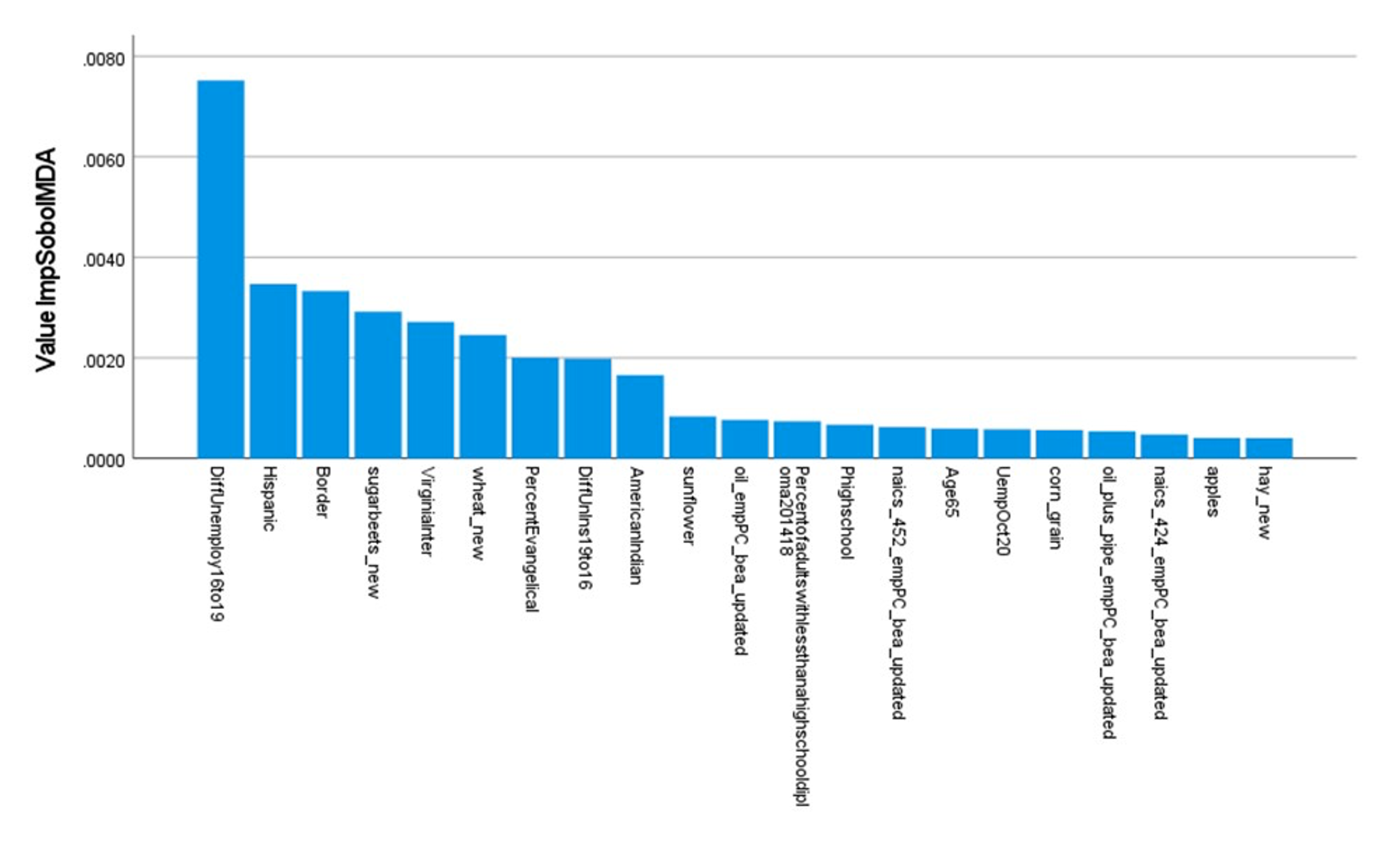
Strikingly, all three programs selected an economic variable identified in our 2020 study as most important for predicting Trump’s vote margin relative to Republican congressional candidates: the county change in unemployment rates between 2016 and 2019. The more unemployment fell, the greater the increase in Trump voting. But the programs disagreed on rankings for other variables, though many were close to each other, and it is unreasonable to expect that programs that work by repeated samples will agree perfectly.
But the differences were hardly negligible, either. We thus proceeded to the next phase of our analysis. We pooled the top twenty variables that each program ranked as most important and considered the whole set in more detail. Appendix Table 1 lists them.
We evaluated the variables using our familiar technique of spatial regressions.23 Once again, for details and references, see our Appendix below as well as our earlier paper. It is only sensible to acknowledge that proceeding in this way comes with a built-in bias toward methodological conservatism. Champions of random forests trumpet the ease with which the method accommodates non-linear relationships of all kinds. Checking results of random forests against the output of spatial regressions is hazardous, because only some forms of non-linearity are readily tested with traditional tools. More complicated combinations resist easy identification.
Researchers need to come to terms with this. We have tried to make due allowance for the point.
Conclusion: The Trump Base and the Persisting Importance of Economic Issues
We are the first to agree that there are plenty of possible reasons to question our results. Our discussion has flagged many points where the inquiry could go off the rails and we will not repeat the litany of cautions again. It should also be obvious from our Appendix, which sets out the full list of variables that we analyzed in the last stage of our inquiry and selected output from the random forest programs we relied on, that one could write a much longer paper about the results. We are planning to do precisely this, but we also think that many issues concerning both methods and results could benefit from further inquiry. This includes the reasons why some variables that often figure in discussions of election results did not make the grade, such as median income, though that particular case is perhaps not perplexing. The same holds for many less familiar variables that appear in Appendix Table 1’s list of the variables selected for further study.
Yet we think our research to date yields a basic finding that is clear and reliable, not just in its own terms, but because it fits with results of other papers. And it can be stated very concisely, by simply moving through the variables in our final model. Here we discuss these non-technically; our Appendix Table 2 sets out and explains in more detail the variables that appear to matter most for catapulting the vote for Trump well over those of Republican House candidates in some districts.
Certain “demographic” variables indeed show as important: Trump’s margin over Republican House candidates ran higher in districts with more Catholics, Hispanics, in districts with more voters whose education stopped with high school, and in counties on the border with Mexico. Counties with higher proportions of older voters also showed more support for Trump than for
Republican congressional candidates. This doesn’t mean that older voters preferred Trump to Biden in general; this gap may well reflect what older voters thought of the much more strident demands by many Republican congressional candidates for fiscal responsibility and even their criticisms of Social Security.24
Our results for Covid’s effects parallel those of our earlier paper for the presidential election, but with a twist. The earlier paper indicated that Covid’s effects varied substantially depending on the number of Trump partisans in districts. Where his support was strong, more people tended to trust the President’s assurances that Covid was really nothing special. By contrast in counties where Trump received less than 40% of the vote, skepticism about the President’s assurances ran much deeper. Higher rates of Covid diminished his vote to a much greater degree.
Trump’s advantage compared to Republican candidates showed analogous switches. High rates of Covid lowered Trump’s margin against Republican congressional candidates everywhere, but the extent to which they did varied markedly. In the high Biden counties, where Republican congressional candidates were less popular to begin with and a vote for the President ran against majority sentiment, the President started out with a larger advantage among stalwarts who stayed with him. But that advantage melted at a higher rate than elsewhere as Covid rates rose.25 Most commentary since the election takes it for granted that Republican voters were relatively unmoved by Covid, rather than simply preferring Trump to Biden in the head-to-head match. Our results suggest that neglect of evidence-based health analyses can be costly even inside the Republican party for the person who is taken to be primarily responsible.
Two variables might be counted as “political.” Trump’s combative responses to mass protests are well known. This perhaps worked to gain him a few votes by comparison with other Republican House candidates, though among all voters it cost him in the general election against Biden.26 The question of whether differences in the expansion of health insurance cost Republicans votes in the presidential election has been debated, unlike the case of 2018, which seems clearer. Our tentative finding is that here, again, the fiscal conservatism typically displayed by Republican congressional candidates did not help them. Trump, by contrast, often dodged responsibility for his party’s and his administration’s efforts to retard healthcare expansion and appears to have benefited from those deceptive moves.27
The rest of the variables are all economic. The agricultural and industrial sectors listed in the table by their numbers in the North American Industrial Classification system are relatively straightforward, though why certain of the industrial sectors turn out to be important is a subject too complicated to discuss here.28 The novelty of the whole line of inquiry calls for extended reflection. This is not political money; in some cases votes might shift for reasons no social scientists have thus far caught, simply because they have hardly looked. Most studies of the mass political effects of specific industries concentrate almost exclusively on cases in which labor was already or was becoming heavily organized. At least up till now, the U.S. is quite far from this situation, though in the past periods of high inflation have eventually led to major labor turbulence.
The remaining economic variables are easier to interpret. As discussed, our earlier paper showed that in counties where rates of unemployment dropped the most, Trump gained votes against Biden. This paper indicates he also gained votes against Republican congressmen and women in those counties. The finding in our earlier paper that in counties where unemployment was especially high in 2020 Trump’s association with economic growth benefited him also holds up here. It advantaged him within his own party.
These results, we think, confirm that Trump’s appeal to his base rests importantly on economic issues, especially economic growth. We repeat that we are not claiming that the economic issues are all that matter: anyone, now, should be able to see how Trump routinely exploits racial and ethnic themes. But the economic appeal is important and not reducible to the others.
As we finished work on this paper, the New York Times published a piece highlighting racial themes that it believed defined Trump’s basic appeal. The article’s test for assessing Trump’s influence was whether Republican members of the House voted to support the challenge to the Electoral College vote on January 6th, 2022. The article was careful: it noted that these districts also showed lower median incomes and lower rates of educational attainment. But it focused on racial prejudice as the key to Trump’s attraction, citing its finding that districts whose representatives voted to support the challenge tended to be districts where the percentage of (Non-Hispanic) whites in the population had declined the most over three decades.29
The Times study compared Congressional districts, not counties, and covered the whole country, not simply districts where Republican candidates mounted serious challenges to Democrats. We readily salute the Times for making the inquiry and find the result very interesting. But our study raises doubts about the uniquely heavy emphasis it places on race.
We are using county data. While county borders change much less over time than congressional districts, some do alter over a generation. But mutations since 2010 are truly minute. Given what is known about how diversity has generally increased across the United States counties since 2010, it seems obvious that if white flight is actually driving the process, then it should show in the time period in which Trump burst on the political scene and won the Presidency. So we tested county rates of change in the white, non-Hispanic percentages of county population between 2010 and 2019 to see if they changed our results. That variable failed to have significance; the other variables continued to work well.
We repeat, again, that this does not mean that racial appeals are not basic to Trump’s appeal to parts of his base. But the result should add plausibility to our claim that economic issues are a separate and very important part of his appeal. As inflation tears into the real incomes of most of the population, this lesson perhaps needs to be absorbed as the driverless car of world history careens to and fro. Otherwise, as the age of electric cars dawns, at least four or more horses and their dreadful riders might someday soon materialize in the sky over Washington, D.C.
Appendix
This Appendix presents our final formal model and technical details of the earlier stages of our research using three different programs for running random forest investigations. This paper relies on the same dataset as our earlier study of the 2020 election, with some obvious updates, such as median income for 2020 instead of 2019 where the substitution makes sense.30 We would call particular attention to Appendix 3 in that paper on the data for industries we use. The industry codes used follow the North American Industry Classification System, but use the data adjusted as per Eckert, et al.31 Alaska is excluded from the dataset, so the number of states is 49.
We begin by describing the outcome variable. This is the difference between Trump’s percentage of the total vote in 2020 and the vote for Republican House candidates mounting substantial campaigns that same year. As our main text explained, our study tried to exclude pure artefacts of the ballot. So we retained districts in which a Republican candidate garnered at least 35% of the total House vote including minor parties, while excluding districts in which the Republican House candidate gained 100% of all votes.
Our analysis then compared how three different random forest programs analyzed 176 covariates of five different types: demographic, geographic, political, economic, and industrial or agricultural sector variables, plus three Covid-19 variables.
We then pooled the top 20 variables selected by each program and analyzed those at length. Descriptive statistics for the variables selected by at least one of the algorithms are listed in Appendix Table 1.
Appendix Table 1:
Descriptive Statistics For Variables Selected For Further Tests
Variable | Mean | Std. Deviation | Min | Max |
Diff Trump Rep House Adj | -1.56 | 5.26 | -57.33 | 33.51 |
Demographic variables: |
|
|
|
|
% Black | 7.86 | 12.22 | 0 | 68.01 |
% Hispanic | 9.22 | 12.93 | 0.61 | 95.19 |
Diff White Non-Hisp 2010- 19 | 2.05 | 1.95 | -9.8 | 19.5 |
% American Indian | 2.00 | 5.96 | 0 | 85.71 |
% Age65 | 19.52 | 4.60 | 4.83 | 57.59 |
% High School but not more | 34.78 | 6.79 | 9.9 | 55.6 |
% Adults with less than HS ed | 13.32 | 6.18 | 1.2 | 66.3 |
% Mormons | 2.34 | 8.90 | 0 | 100.79 |
% Evangelical | 23.65 | 16.33 | 0 | 130.87 |
% Catholic | 11.97 | 12.84 | 0 | 99.96 |
Pct Diff in Total Pop 2019 to2010 | 0.01 | 0.09 | -0.34 | 1.34 |
Geographical Variables: |
|
|
|
|
Border | 0.01 | 0.11 | 0 | 1 |
Virginia Counties Interpolated | 0.02 | 0.12 | 0 | 1 |
Socioeconomic Status |
|
|
|
|
Median Income 2020 | 56.97 | 13.30 | 22.90 | 155.36 |
Uemp Oct20 | 5..08 | 1.99 | 1 | 18.2 |
Diff Unemploy2016to19 | 1.26 | 1.01 | -1.6 | 8.9 |
Diff Health Insurance % 2019to16 | 0.89 | 1.34 | -6.98 | 7.82 |
Political Variables |
|
|
|
|
Heavy Polluting Industries | 4.48 | 5.13 | 0 | 56.37 |
Protest Princeton Index | 4.68 | 13.16 | 0 | 168 |
High Biden vote counties | 0.03 | 0.18 | 0 | 1 |
Covid-19 |
|
|
|
|
% Covid | 2.95 | 1.75 | 0.07 | 17.19 |
CovidbyHighBiden Interaction | 0.10 | 0.63 | 0 | 13.61 |
Interaction Protest by %Hispanic | 68.41 | 355.23 | 0 | 9806.43 |
Industry |
|
|
|
|
alfalfa | 0.07 | 0.13 | 0 | 1 |
apples | 0.00 | 0.01 | 0 | 0.28 |
hay_new | 0.28 | 0.31 | -0.80 | 1.00 |
corn_grain | 0.17 | 0.19 | 0 | 0.79 |
corn_silage | 0.02 | 0.04 | 0 | 0.40 |
sugarbeets_new | 0.00 | 0.01 | 0 | 0.24 |
sunflower | 0.00 | 0.01 | 0 | 0.20 |
soybeans | 0.16 | 0.18 | 0 | 0.64 |
wheat_new | 0.10 | 0.17 | 0 | 0.92 |
naics_52 | 1.85 | 1.26 | 0 | 22.78 |
naics_424 | 1.09 | 1.36 | 0 | 38.24 |
naics_447 | 1.16 | 0.82 | 0 | 10.05 |
naics_451 | 0.16 | 0.21 | 0 | 2.50 |
naics_452 | 1.59 | 1.17 | 0 | 9.59 |
naics_624 | 1.36 | 1.25 | 0 | 27.47 |
naics_713 | 0.62 | 1.43 | 0 | 33.51 |
naics_722 | 4.65 | 2.18 | 0 | 26.73 |
naics_812 | 0.40 | 0.31 | 0 | 5.12 |
naics_813 | 1.29 | 0.71 | 0 | 12.90 |
Oil_plus_pipelines | 0.52 | 1.91 | 0 | 28.65 |
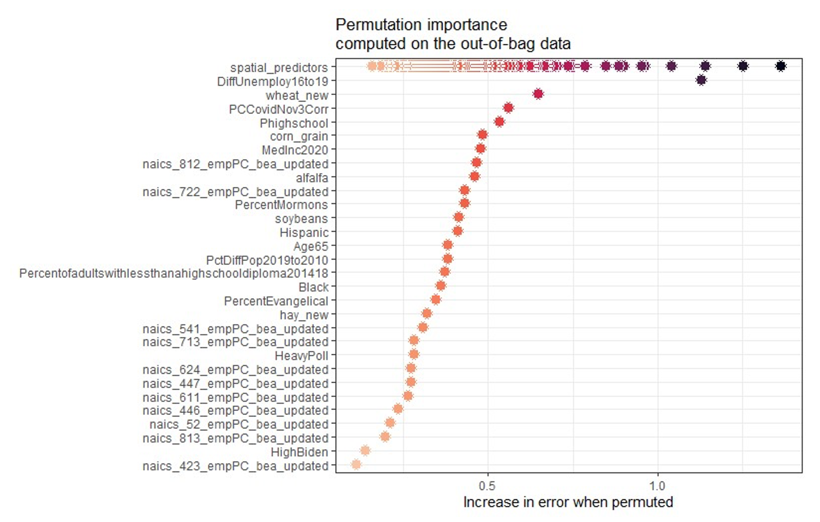
The first random forest program we used was the R package spatialRF developed by Benito (2021).32 This program uses the faster Random Forest R package ranger developed by Wright and Ziegler with spatial predictors to generate Moran eigenvector maps (MEMs) from a distance matrix.33 MEMs are ranked using Moran’s I. Spatial predictors are included in the model until the spatial autocorrelation of the residuals becomes neutral. These spatial predictors can be saved and used in other random forest models. The twenty most important variables the program selected are shown in Appendix Figure 1 and their Partial Dependent Plots (PDP) are shown in Appendix Figure 2. The importance measures were calculated based on the increase in mean error from out-of-bag data across trees when a predictor is permuted.
Appendix Figure 1:
Example of Variables Importance, Spatial Model
Appendix Figure 2:
Partial Dependent Plots – Spatial Model
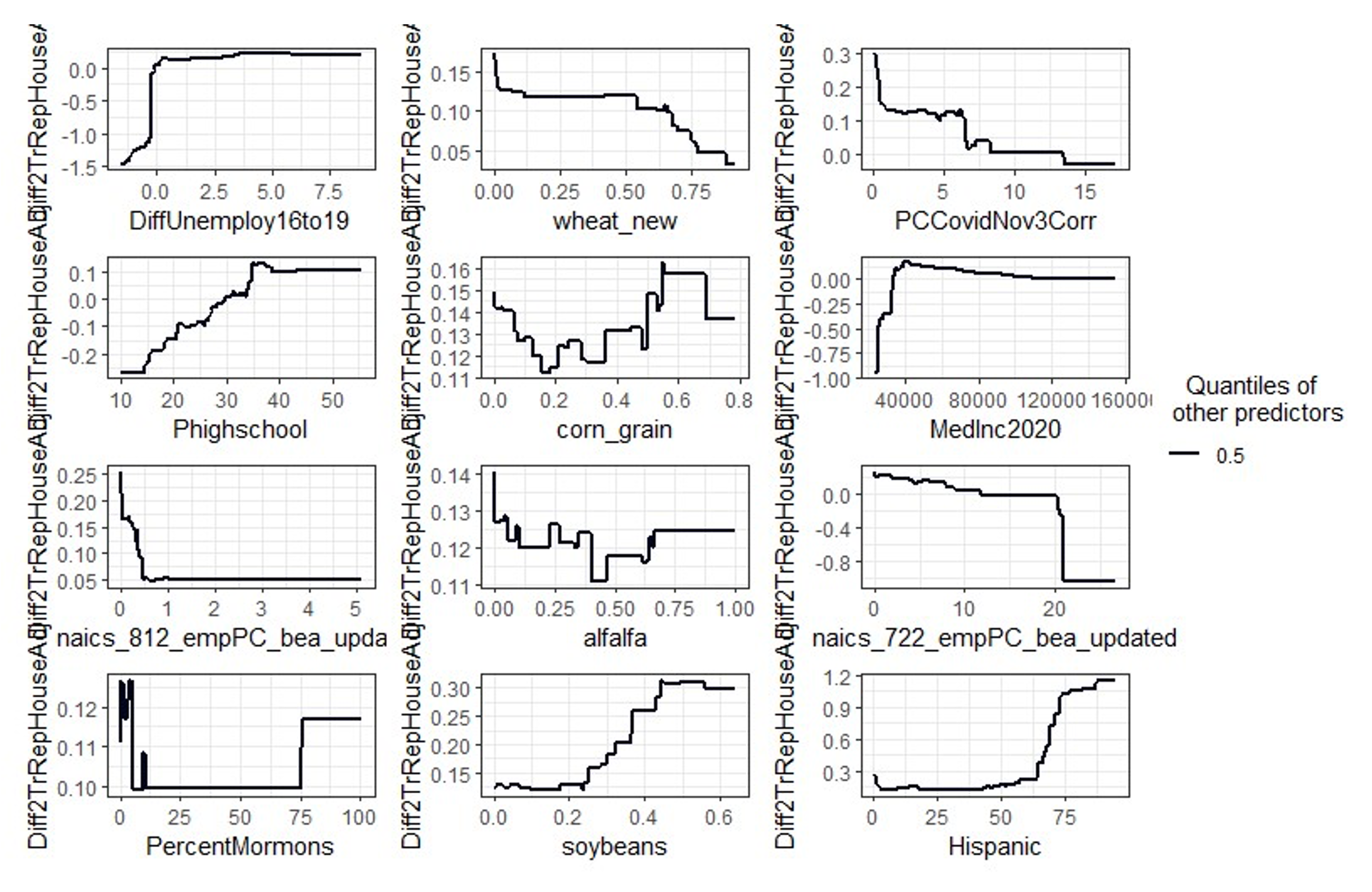
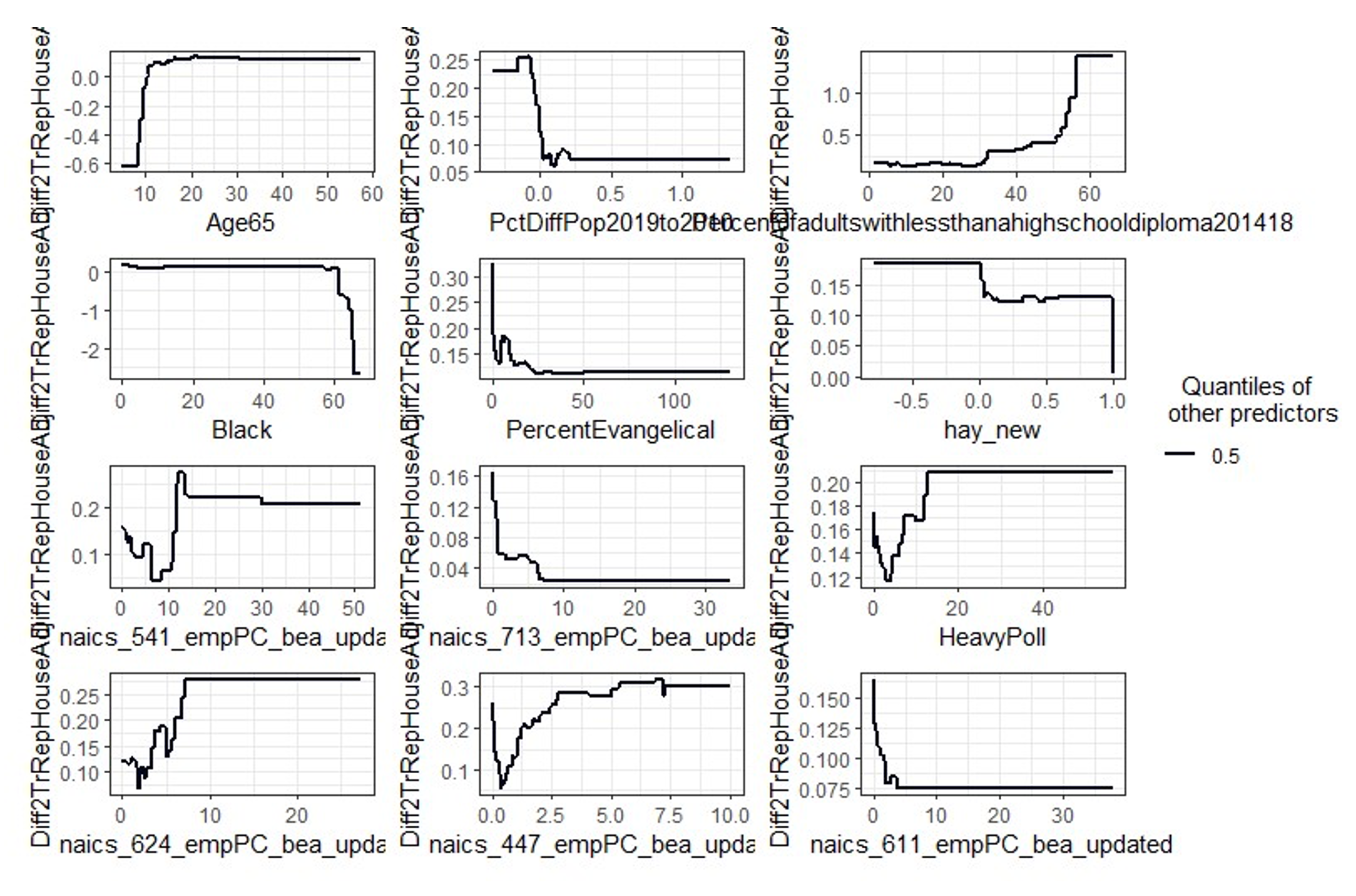
Following the approach in SpatialRF, we used the saved spatial predictors from spatialRF in the other two programs used, BorutaShap and SobolMDA.
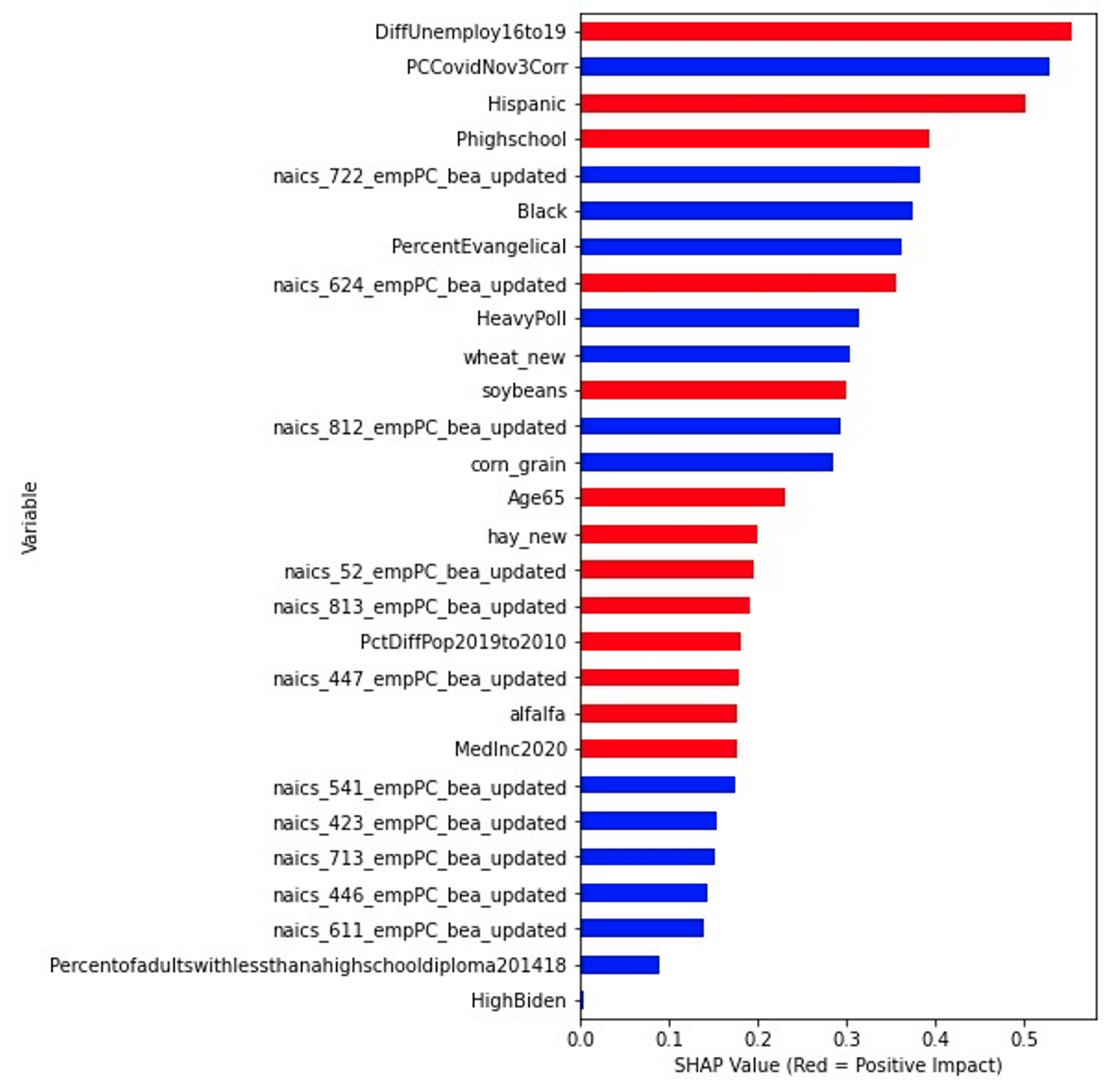
The BorutaShap Python package combines the Boruta algorithm with Shapley values (Lundberg, S. M., and Lee, S. I. 2017). Spatial predictors are included in the models. The SHAP feature importance results are displayed in Appendix Figures 3 and 4. Figure 3 is SHAP Summary Plot and Figure 4 is SHAP feature importance plot in which a red color indicates the positive association with the outcome variable (Trump’s margin compared to Republican House candidates) and blue a negative impact. SHAP dependence plots are an alternative to partial dependence plots. SHAP dependence plots display a variable’s variance on the y-axis, and can be colored with another variable to show the interaction. Note that the variables selected by each program are not the same; that is precisely why we proceed as we do in this paper.
Appendix Figure 3:
SHAP summary Plot, variables are ordered according to their importance.
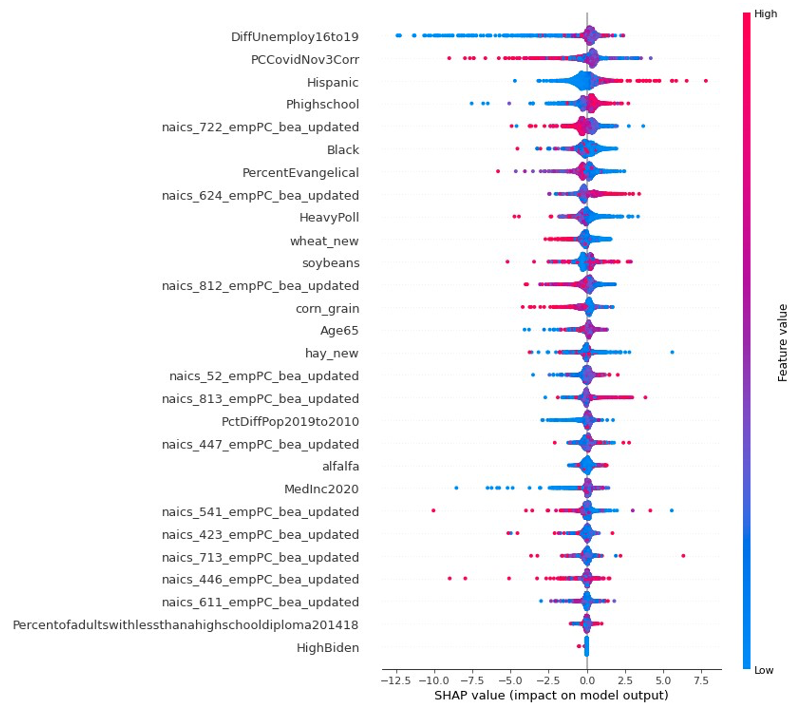
Appendix Figure 4:
SHAP Summary Plot: Color Indicates Variable Direction
The third algorithm we used is the Sobol-Mean Decrease Accuracy (SobolMDA) measure developed by Bernard, Vega, and Scornet.34 A form of sensitivity analysis, it is designed to calculate consistent estimates of the total Sobol index based on the reduction of explained variance.
We then analyzed all the selected variables using a spatial regression model; we report only significant (p-v < .05) and marginally significant (p-v < .10) variables in Appendix Table 2. From many previous efforts, we expected to find strong spatial correlation in our data. Spatial autocorrelation is quite like temporal autocorrelation; they both make trouble in statistical analysis. The customary method for detecting spatial autocorrelation is a Moran test. Our tests showed that spatial autocorrelation was indeed present, so we switched from ordinary least squares regression to spatial error regression based on Lagrange Multiplier tests.35
Table 2 presents the estimated spatial regression coefficients; that table also shows the coefficients computed from an ordinary least squares regression (OLS).
Appendix Table 2:
Model Fixed Effect OLS and Spatial Error Model
| OLS Model | Spatial Error |
|
|
Intercept | -5.87 (0.00) | -11.26 | (0.00) |
|
Demographic Variables |
|
|
|
|
% Hispanic | 0.63 (0.00) | 0.04 | (0.00) |
|
% high school | 0.54 (0.00) | 0.10 | (0.00) |
|
% Age65 | 0.22 ( 0.02) | 0.04 | (0.04) |
|
% Catholic | 0.23 (0.03) | 0.01 | ( 0.09) |
|
Border (Yes vs. No) | 2.88 (0.00) | 2.36 | (0.01) |
|
Virginia Inter (Yes vs. No) | -4.87 (0.00) | -2.83 | ( 0.00) |
|
Socioeconomic Status |
|
|
|
|
DiffUnemploy16to19 | 0.23 (0.04) | 0.23 | (0.02) |
|
DiffUnIns19to16 | 0.27 (0.00) | 0.13 | (0.01) |
|
Election |
|
|
|
|
HighBiden | 2.48 0.00) | 2.48 | (0.00) |
|
ProtestPrincea | 0.13 (0.16) | 0.01 | (0.04) |
|
% Cov19Nov3 by populationb | -0.37 (0.00) | -0.10 | ( 0.04) |
|
Industry and Agriculture |
|
|
|
|
sugarbeets_new | 0.34 (0.00) | 16.04 | (0.02) |
|
hay_new | -0.08 (0.45) | 0.63 | (0.06) |
|
corn_grain | -0.45 (0.00) | -1.58 | (0.07) |
|
sorghum | -0.01 (0.88) | -3.93 | (0.07) |
|
naics_722 | -0.41 (0.00) | -0.11 | (0.00) |
|
naics_812 | 0.01 ( 0.92) | -0.57 | (0.01) |
|
Interaction |
|
|
|
|
CovidbyHighBiden | -0.66 (0.00) | -1.10 | (0.00) |
|
N | 2874 |
| 2874 | |
R2/Nagelkerke pseudo-R2 | 0.43 |
| 0.63 |
a: Data source is the Armed Conflict and Event Location Project, as explained there.
b: Accumulated Covid-19 cases since the beginning to Nov 3, 2020. Percent Population
Like the model in our earlier 2020 paper, this final model is a spatial version of a fixed effect general linear model. It includes separate intercepts for each state to take account of heterogeneity between them.
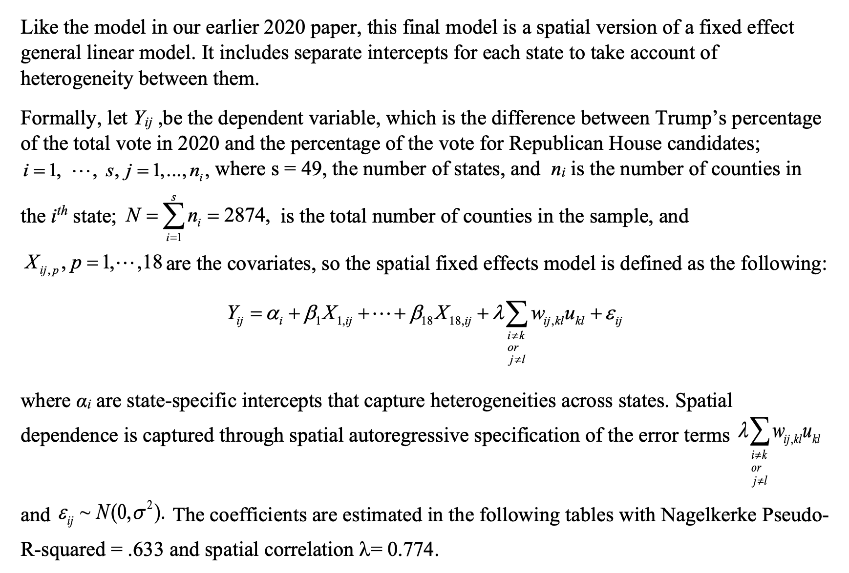
The coefficients on the variables can be interpreted as follows:
The estimated coefficient for the percent of Hispanic is .04 (p-v = .00). For every 1% increase in the percentage of Hispanics in the county, Trump’s expected change of votes compared to the Republican House candidate is increased by 0.04%.
The estimated coefficient for the percent of High School graduates (but no further educational experience) is .10 (p-v = .00). For every 1% increase of PHighschool, Trump’s expected change of votes compared to Republican House candidates increases by .10%.
The estimated coefficient for the Age65 is .04 (p-v = .04). For every 1% increase in the percentage of the county population aged 65 and over, Trump’s expected change of votes compared to Republican House candidates increases by .04%.
The estimated coefficient for the Percent of Catholic is .01 (p-v = .09). For every 1% increase in the Catholic percent of the county population, Trump’s expected change of votes compared to Republican House candidates increases by .01%.
The estimated coefficient for Border is 2.36, compared with non-border counties; Trump’s expected change of votes compared to Republican House candidates is 2.36% higher for border counties. Border counties are defined as in (Ferguson et al., 2021).
The estimated coefficient for VirginiaInter is -2.83, compared with other counties in Virginia; Trump’s expected change of votes compared to Republican House candidates is 2.83% lower in those counties. This variable is included only because we had to interpolate some data for a small subset of Virginia counties for reasons peculiar to the way their data is reported. The issues we think are irrelevant to this paper, but we include the variable anyway. In those counties, Trump fared rather worse than elsewhere.
The estimated coefficient for the percent difference of unemployment from 2016 to 2020 is .23 (p-v = .02). For every 1% decrease in the unemployment rate from 2016 to 2020, Trump’s expected change of votes compared to Republican House candidates is increased by 0.23%.
The estimated coefficient in the change in the percent of the population insured [for health care] between 2016 and 2019 is .13 (p-v = .01). For every 1% increase in the insured rate from 2016 to 2019, Trump’s expected change of votes compared to Republican House candidates increases by 0.13%. See the discussion in our main text but also our earlier paper on data issues.
HighBiden, % Cov19Nov3 by population, and the interaction of these two variables
CovidbyHighBiden are used together to better estimate Covid’s real effect on the 2020 election. The problem is outlined in our main text and at much greater length in section 3 of our earlier paper. % Cov19Nov3 by population is exactly what its name implies: the cumulative percent of the population in counties that had contracted Covid as of election day, 2020. But Covid’s effect varies dramatically depending on how heavily counties voted for Trump. In High Biden counties (where Trump garnered less than 40% of the vote), the President’s dismissals of Covid were much less widely accepted and high rates of Covid cost him much more heavily against Biden, as shown in (Ferguson et al., 2021). That result, though, implies that the voters who stuck with the Trump in High Biden counties were likely more stalwart, while Republican congressional candidates were less popular to begin with. This explains the initial positive coefficient in Trump’s favor compared to Republican congressmen and women in High Biden counties at zero rates of Covid. But in those, his advantage against Republican candidates dropped sharply as Covid rates rose. The estimated coefficient for HighBiden is 2.48 (p-v = .00) for counties with no Covid19 Cases. As Covid spreads in the High Biden counties, Trump’s expected change of votes compared to Republican House candidates decreases by 1.20%, while in the rest (low Biden) counties, his expected change of votes compared to Republican House candidates decreases by only .10%.
The estimated coefficient for ProtestPrince is .01 (p-v = .04). For every increase in protests events,Trump’s expected change of votes compared to Republican House candidates increases by 0.01%.
The estimated coefficient for sugarbeets_new is 16.04 (p-v = .01). For every 1% increase in the percentage of sugarbeets_new in a county’s agricultural production, in Trump’s expected change of votes compared to Republican House candidates is increased by 16.04%.
The estimated coefficient for hay_new is .63 (p-v = .06). For every 1% increase in the percent of hay_new, in a county’s agricultural production, Trump’s expected change of votes compared to Republican House candidates increased by 0.63%.
The estimated coefficient for corn_grain is -1.58 (p-v = .07). For 1% increase in the percent of a county’s agricultural production of corn_grain, Trump’s expected change of votes compared to Republican House candidates decreased by 1.58%.
The estimated coefficient for sorghum is -3.93 (p-v = .07). For every 1% increase in a county’s total agricultural production of sorghum, Trump’s expected change of votes compared to Republican House candidates decreased by 3.93%.
The estimated coefficient for naics_722 is -.11 (p-v = .00). For every 1% increase in the percent of total county employment in the industry naics_722, Trump’s expected change of votes compared to Republican House candidates is decreased by .11%.
The estimated coefficient for naics_812 is -.57 (p-v = .001). For a 1% increase in the percentage of county employment of naics_812, Trump’s expected change of votes compared to Republican House candidates decreases by .57%.
References
Angrist, J., & Frandsen, B. (2019). Machine Labor. National Bureau of Economic Research, Working Paper Number 26584. Retrieved from https://www.nber.org/papers/w2…
Anselin, L. (2002). Under the Hood: Issues in the Specification and Interpretation of Spatial Regression Models. Agricultural Economics, 27(3), 247-267.
Athey, S., & Imbrens, G. W. (2019). Machine Learning Methods Economists Should Know About. In Annual Review of Economics Vol. 11 (pp. 685-725).
Bénard, C., Da Veiga, S., & Scornet, E. (2022). Mean Decrease Accuracy for Random Forests: Inconsistency, and a
Practical Solution via the Sobol-MDA. Biometrika. Retrieved from https://doi.org/10.1093/biomet…
Benito, B. (2021). spatialRF: Easy Spatial Regression with Random Forest. R package. Retrieved from https://blasbenito.github.io/s…
Breiman, L. (2001). Random Forest. Machine Learning 45, 5-32. Retrieved from http://dx.doi.org/10.1023/A:10…
Cavallaro, M. (2021). Local David Versus Global Goliath: Populist Parties and the Decline of Progressive Politics in
Italy Institute for New Economic Thinking Working Paper No. 80. Retrieved from https://www.ineteconomics.org/…
CNBC. (2022, October 6, 2022). Biden: Nuclear ‘Armageddon’ Risk Highest Since ’62 Crisis. CNBC. Retrieved from https://www.cnbc.com/2022/10/0…
Debeer, D., & Strobl, C. (2020). Conditional Permutation Importance Revisited. BMC Bioinformatics, 21. Retrieved from. https://doi.org/10.1186/s12859…
Dray, S., Legendre, P., & Peres-Neto, P. R. (2006). Spatial Modeling: A Comprehensive Framework for Principle Coordinate Analysis of Neighbor Matrices (PCNM). Ecological Modeling 196(3-4), 483-493. Retrieved from https://doi.org/10.1016/j.ecol…
Eckert, F., Fort, T. C., Schott, P. K., & Yang, N. J. (2021). Imputing Missing Values in the US Census Bureau’s County Business Patterns National Bureau of Economic Research Working Paper No. 26632; retrieved from: https://www.nber.org/papers/w26632.
Ferguson, T. (1995). Golden Rule: The Investment Theory Of Party Competition And The Logic Of Money-Driven Political Systems. Chicago: University of Chicago Press.
Ferguson, T., Jorgensen, P., & Chen, J. (2021). The Knife Edge Election of 2020: American Politics Between Washington, Kabul, and Weimar, Institute for New Economic Thinking Working Paper No. 169; Retrieved from https://papers.ssrn.com/sol3/p…
Ferguson, T., Page, B., Rothschild, J., Chang, A., & Chen, J. (2020). The Roots of Right-Wing Populism: Donald
Trumpin 2016. International Journal of Political Economy, 49, 102-123. Retrieved from https://www.tandfonline.com/do…
Gaspard, P., Greenberg, S. B., Lake, C., & Lux, M. (2022). A Memo to Democrats. The American Prospect.
Retrieved from https://prospect.org/politics/…
Griffth, D. A., & Peres-Neto, P. R. (2006). Spatial Modeling in Ecology: The Flexibility of Eigenfunction Spatial
Analyses. Ecology, 87, 2603-2613. Retrieved from https://doi.org/10.1890/001296…
Hengl, T., Nussbaum, M., Wright, M., Heuvelink, G., & Gräler, B. (2018). Random Forest as a Generic Framework for Predictive Modeling of Spatial and Spatio-Temporal Variables. PeerJ 6:e5518. Retrieved from https://doi.org/10.7717/peerj….
Keller, M. H., & Kirkpatrick, D. D. (2022, Updated October 27). Their America Is Vanishing. Like Trump, They
Insist They Were Cheated. New York Times. Retrieved from
https://www.nytimes.com/2022/1…
Kou, C. (2019). Explain Your Model With the SHAP Values. Medium. Retrieved from https://medium.com/dataman-in-…
LeSage, J., & Pace, R. K. (2009). Introduction to Spatial Econometrics. Boca Raton: Chapman & Hall/CRC Press.
Mullainathan, S., & Spiess, J. (2017). Machine Learning: An Applied Econometric Approach. Journal of Economic Literature, 31(2), 87-106.
Saha, A., Basu, S., & Datta, A. (2021). Random Forests for Spatial Dependent Data. Journal of the American
Statistical Association, 2021. Retrieved from https://doi.org/10.1080/016214…
Shiffrin, R. M. (2016). Drawing Causal Inference From Big Data. Proceedings of the National Academy of Science,
113(27), 7308-7309. Retrieved from www.pnas.org/cgi/doi/10.1073/p…
Strobl, C., Boulesteix, A.-L., Kneib, T., Augustin, T., & Zeileis, A. (2008). Conditional Variable Importance for
Random Forests. BMC Bioinformatics, 9(307). Retrieved from doi:10.1186/1471-2105-9-307
Wright, M. N., & Ziegler, A. (2017). Ranger: A fast implementation of random forests for high dimensional data in C++ and R. Journal of Statistical Software, 77(1). Retrieved from http://dx.doi.org/10.18637/jss…
Notes
The authors are very grateful to Blas Benito and Clément Bénard for very helpful and timely responses to questions.
Thanks also to Charles Delahunt and Shawn McGuire for early encouragement and to the Institute for New Economic Thinking for support that made it possible for us to run two machines at once. Thanks also to Pia Malaney for comments on the manuscript and Zihan Li and James Hershman for other helpful advice
1 See, e.g., (CNBC, 2022).
2 (Gaspard, Greenberg, Lake, & Lux, 2022) among many sources.
3 For the scholarly discussion, see the references in (Ferguson, Jorgensen, & Chen, 2021) and (Ferguson, Page, Rothschild, Chang, & Chen, 2020). The Times piece is (Keller & Kirkpatrick, 2022).
4 2018’s extraordinary turnout, reminiscent of a presidential election, suggests that something may be changing in the political system.
5 By including Republican candidates who have little or no chance of winning, it may also send investigators down a false trail if the real question is Trump’s position vis a vis Republican congressmen and women.
6 (Ferguson et al., 2021).
7 (Ferguson et al., 2020) for 2016; for an Italian case cf. (Cavallaro, 2021).
8 We treat agricultural sectors as special cases of a broad “industrial” structure, as our paper explained. 9 (Ferguson et al., 2021). The point applies, too, discussions of Trump’s margins compared to other Republican candidates. Party line voting should not be assumed regardless of all the talk of increased partisanship.
10 We caution about claims that individuals vote on only one or two issues. They don’t, and nothing in this paper assumes they do. But when a broad issue like economic decline affects large numbers of people, the pros and cons of candidates and parties as voters perceive them will change broadly. See the discussion in (Ferguson, 1995), esp.
the Appendix, but also the empirical evidence of voters’ misgivings about Trump in (Ferguson et al., 2020).
11 Methods for analyzing natural language texts are becoming much more common, even if many problems remain.
12 The literature is copious; see, e.g., (Athey & Imbrens, 2019); (Mullainathan & Spiess, 2017). Specifically on instrumental variables, where a possible use for them is recognized see, e.g., (Angrist & Frandsen, 2019), which offers many cautions. On causal explanations, see the succinct statement of problems in (Shiffrin, 2016).
13 See the discussion in (Ferguson et al., 2021); technically the phenomenon is an example of “rationalization” where some voters adopt the issue stance of a candidate they trust.
14 Various papers sought to solve the problem by means of an instrumental variable. They chose meat packing as the variable. (Ferguson et al., 2021) explains why the use of that introduces new errors. The solution we advanced is not perfect either, but it does not stray as far from reality as other solutions.
15 Cf. (Shiffrin, 2016): comments that “However, there are enormous difficulties facing researchers trying to draw causal inference from or about some pattern found in Big Data: there are almost always a large number of additional and mostly uncontrolled confounders and covariates with correlations among them, and between them and the identified variables. This is particularly the case given that most Big Data are formed as a nonrandom sample taken from the infinitely complex real world: pretty much everything in the real world interacts with everything else, to at least some degree.” One is reminded of Hegel’s famous dismissal of Schelling’s Absolute as a night in which all cows are black.
16 The danger of “overfitting” models with too many variables is heavily stressed in traditional statistics. See (Athey & Imbrens, 2019); a lucid discussion of the contrasting approaches is (Bénard, Da Veiga, & Scornet, 2022). See also the seminal early paper by (Breiman, 2001).
17 (Athey & Imbrens, 2019); the quotation continues: “even if the assumption that the underlying process is at least approximately sparse is still a strong one, and even if inference in the presence of data-dependent model selection can be challenging.”
18 The literature is very large. (Strobl, Boulesteix, Kneib, Augustin, & Zeileis, 2008) was a particularly helpful early critique. See also (Debeer & Strobl, 2020).
19 See, e.g., (Bénard et al., 2022) or (Kou, 2019).
20 (Benito, 2021).
21 (Bénard et al., 2022).
22 (Dray, Legendre, & Peres-Neto, 2006); (Griffth & Peres-Neto, 2006); (Hengl, Nussbaum, Wright, Heuvelink, & Gräler, 2018). An interesting application is (Saha, Basu, & Datta, 2021).
23 The spatial regressions followed the pattern of our 2020 paper: These use spatial contiguity as the basis for the spatial matrix and included a set of fixed effects variables for states.
24 Our Appendix Table includes a term for a few counties in Virginia and indicates these were less friendly territory for Trump. They are singled out simply because data peculiarities specific to some federal tabulations for that state required us to interpolate a few entries. None of the details matter for this paper, but we left the term in for completeness.
25 The use of the interaction in preference to a more usual instrumental variable for assessing Covid’s effect is explained in (Ferguson et al., 2021), section 3. The positive sign for the High Biden districts almost surely means that the voters who did cast votes for Trump liked him better than Republican House candidates running in their district, which is hardly a surprise.
26 (Ferguson et al., 2021).
27 We take it as a given that the Trump administration in fact strongly opposed extending health insurance, but that Trump usually tried to duck responsibility for the decisions. In the 2016 he clearly dodged such questions. Cf. (Ferguson et al., 2020). Republican congressmen and women, by contrast, we believe were much clearer about their views.
28 Some of the agricultural sectors are fairly obvious; Trump’s administration killed planned reports on the dangers of some crops, for example. More another time. It is worth noting that heterogeneity within some industrial sectors can be important.
29 (Keller & Kirkpatrick, 2022).
30 (Ferguson et al., 2021).
31 (Eckert, Fort, Schott, & Yang, 2021).
32 (Benito, 2021).
33 For Ranger, see (Wright & Ziegler, 2017); for the distance matrix approach cf. (Dray et al., 2006) and (Hengl et al., 2018).
34 (Bénard et al., 2022).
35 (Anselin, 2002); (LeSage & Pace, 2009).