The Straight Truth
The 2020 election and the cataclysmic series of events it triggered have left many Americans dazed and sometimes even breathless. Not the least of these shocks stems from the Democrats’ unexpectedly poor showing in Congressional races. While narrowly winning the presidency, the party actually lost seats in the House and failed in its bid to take control of the Senate. The disappointment – or relief for Republicans – was all the greater in that in the weeks before the election, virtually every major media outlet pushed out stories trumpeting what was said to be overwhelming Democratic advantages in fundraising – more than twenty, by our incomplete count.
The morning after the election, though, the press flip-flopped. No one stopped to wonder if the mid- and late-October pre-election counts were misleading or simply wrong. Instead, the major media ran story after story highlighting the extravagance of strong claims about the money-driven character of American elections. Reporters celebrated how canny voters in Maine and other states saw through the clouds of out of state big money. Our favorite summary – it should be enshrined forever in the Madame Tussaud’s of hasty social science misjudgments – was a tweet by Edward Luttwak that “The very good news of 2020: money does not win elections in America. Because of the proclivities of American billionaires, Democratic candidates had x2 or x3 or x4 the money of Republicans in House, Senate & WH elections. Holder, Obama’s AG spent hugely in States but Dems lost.”
Last year’s presidential race is sui generis and fraught with chilling lessons for the future of American politics. We will analyze it carefully another time. Our concern here is with the Congressional elections. In contrast to presidential runs, races for the House and Senate are not one-offs. The hundreds of cases permit real generalizations.
Before the election, when we were asked, we cautioned about claims of a one-sided Democratic advantage. We did not doubt the stories drawing on partial, pre-election fundraising reports, testified to strong Democratic fundraising efforts. Nor, though we wondered about the margins, did we doubt that the Democrats were probably then ahead in the polls.
But we have tracked money and politics through many election cycles. We knew the flows of money streaming into campaigns in the final weeks of elections are often gigantic. The epic, come from behind struggle in 2016 to salvage Republican control of the Senate was also fresh in our minds, since we had just published a study which analyzed it in detail.
That effort’s defining feature was a rip tide of late money that turned around what looked like a hopeless situation when most observers believed their party’s presidential standard bearer was doomed. In 2020, signs that similar efforts might be afoot were obvious. In Maine, for example, in mid-October, a single private equity magnate dropped his third contribution of $500,000 dollars in the election cycle into a single candidate super-PAC supporting Republican Senator Collins.
We were confident that our “linear model” of House and Senate races – so-called because the relation between the two-party split of the money and the outcome of the vote looks like a straight line when you plot it – would prove out, as it had in every previous election for which the data exists to compute it. And we doubted that trailing in the polls would put off many big Republican contributors, any more than in 2016. The whole point of our work is that most money rarely follows polls.
Figures 1 and 2 confirm we were right. At a moment, when everything appears to be up for grabs in American politics, some things have not changed: the system is still money-driven.
Do not be put off by the figures. They are simple scatter diagrams and easy to read. Along the bottom from left to right runs the Democratic percentage of the total amount spent on any given race – not the cost of votes per ballot or other measures that vary with district size and other characteristics. The vertical axis going up the left side benchmarks the percentage of the two-party vote that the Democrats garner. That axis is scaled as the difference between the Democratic and Republican shares of the vote, meaning that as the difference goes positive for the Democrats (roughly in the middle of the figure), they start winning seats. At the bottom left corner, in other words, the Democrats get no or hardly any money and win no or hardly any seats. At the upper right, they slurp in all the money and get all the votes.
The spread of the dots around the line – outcomes of actual races – shows how far reality diverged from the pure linear model. The discordance in 2020, as in so many elections before, was not much. Some races did deviate – they always do, and last year Democrats lost some close ones they might normally have won. But the big story is the continued dominance of the linear model. The best ways to summarize the model’s strength are highly technical, because in the House, almost always, and sometimes in Senate races, you need to take account of various races’ spatial relationships to each other. We tuck the details in our Appendix here, along with a brief explanation of how to show up the perennial last hope of orthodox political science and economics, that seeing cannot be believing, because the money must be following polls.)
Noam Chomsky has recently remarked that there are few real regularities discovered in the social sciences, but that the linear model is one.[1] After forty years of evidence, it’s time to agree and move on. The next time you wake up to find that election results in hundreds of Congressional elections differ wildly from what you would expect from the reported division of political money, check more carefully whether the voice of the people is not really the sound of money talking. And if you are trying to understand why both major parties instantly acquiesce to whatever it takes to rescue financial markets and the 1%, but fight over relief for the rest of us, you have the major part of the answer. The basic root of K-shaped recoveries is the hold political money has on both major political parties.
Appendix: Models, Methods, and Data
All our methods and data sources are spelled out at length in the Appendices to Thomas Ferguson, Paul, Jorgensen, and Jie Chen, “How Money Drives US Congressional Elections: Linear models of Money and Outcomes,” Structural Change and Economic Dynamics 2019.
For 2020, as usual, we gathered all candidate disbursements and outside money from any source spent in support of the candidate, including negative advertising against opponents, to construct the percent of all money favoring the Democratic candidate in each House and Senate election. The campaign spending data derives from multiple Federal Election Commission datasets, containing candidate summary spending totals, independent expenditures (from Super PACs and dark money groups), party coordinated expenditures, electioneering communications (which we examine to clearly identify the support of or opposition to candidates), and communications costs (campaigning internal to some corporations and unions). Note that these include “dark money” totals, but not its real sources. The voting data come from David Leip’s Atlas of U.S. Presidential Elections.
For our models we drop races without two major party candidates; see our Structural Change and Economic Dynamics discussion. In many cases, those are best viewed as auctions. We always test for spatial autocorrelation in races. This is often present in House elections and sometimes for Senate elections. We include the final outcomes of the Georgia Senate races on our Figure 2, but since they were stand alones on a different day, not for calculating the model fit.
The strong linear character of the model, which holds for all elections for which data exists, has been a standing embarrassment to voter centered accounts of politics from the moment it was published. Many critical responses are simply silly; they don’t pay enough attention to details. But we take the force of the objection that in theory, the money could be following polls, in whole or in part, making the apparent correlation spurious.
The usual social science device to deal with questions of “endogeneity” is some form of instrumental variable. Those are often highly problematic. In our earlier work, we developed a spatial version of the latent instrumental variable model introduced by Peter Ebbes and analyzed in detail by Irene Hueter to assess such possibilities. Our Structural Change piece discusses these, but in addition shows how to use published gambling odds to confirm our conclusions that while two-way causality happens, it does not dominate; the 2016 Republican Senate recovery was a particularly dramatic case in point. Note that since we developed the linear model, other researchers find evidence for it in other countries; the pattern is not specific to the United States.
Our presentation of results here follows that in our longer essay. As usual, the House elections showed marked spatial autocorrelation based on a Moran I test. This indicated that the residuals of the OLS model displayed significant spatial dependence (PV(I) < .001). For the House we thus report, successively, results using ordinary least squares, then a spatial Durbin model, followed by the Bayesian spatial latent instrumental variable regression with 4 clusters we prefer, along with R squared and Pseudo R squared measures first for the OLS and then the spatial model, followed by a test for spatial effects and then N, the number of cases. Figure 1 showing results for the House displays the Pseudo R squared measure for the spatial model, since the Bayesian spatial latent instrumental model does not have such a convenient summary indicator.
House
Year | OLS | Spatial Model | SBLIV4 | RSq/PRSq | PV(I) | N |
2020 | .825(.023) | .718 (.023) | .731(.679,.781) | .759/.810 | .000 | 404 |
Spatial models were unnecessary for the Senate elections, so the table does not show any. We present results for the OLS model and for a Bayesian latent instrumental variable regression with 3 clusters.
Senate
Year | OLS Coefficients ( SE) | BLIV3 Median ( 95% CI ) | R-square | N |
2020 | .732 (.074) | .729(.587,.873) | .761 | 33 |
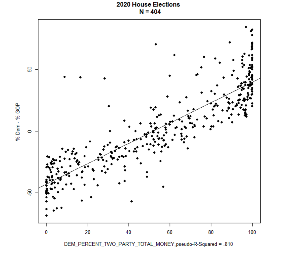
Figure 1: The Straight Truth: Money and Major Party Votes in the House Data: Money From the FEC; Votes from Leip’s Atlas of U.S. Presidential Elections
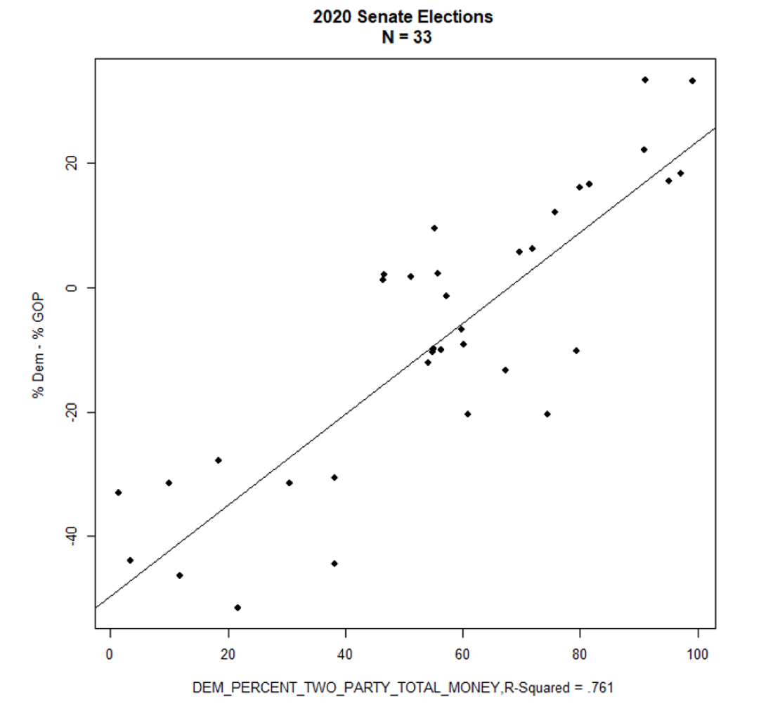
Figure 2: The Straight Truth: Money and Votes in the Senate Data: Money From the FEC; Votes from Leip’s Atlas of U.S. Presidential Elections Display Includes the Special Senate Elections in Georgia in January, Though They Are Not Included in the Summary Statistics – See Appendix