The third and final round of response from Andrew Smithers on Lance Taylor’s INET working paper on the alleged “global savings glut.”
My previous comment, in summary, was as follows:
(i) Professor Taylor chooses to ignore rather than dispute my point that the labour and capital shares of output, which together add up to 100%, must be measured in a comparable way in accordance with the definition of income set out in Value and Capital: An Enquiry into Some Fundamental Principles of Economic Theory by J.R. Hicks Oxford University Press (1939). As the point is not disputed I take it that it is accepted.
(ii) The data on the profit share of corporate output are available from 1929, but Professor Taylor does not use them. He restricts his series to the data after 1970, thus ignoring the previous 41 years. This is contrary to the important principle that in order to avoid “data mining” all available data should be used.
In his reply to my first point Professor Taylor writes that “Andrew Smithers seized on measures of profits, but that was not the key point that requires elucidation. For a business, profits are a residual, equaling revenues minus costs. This observation carries over to the national income and product accounts constructed by the US Bureau of Economic Analysis (BEA). It makes sense to look at how shaky the BEA estimates of profits really are.”
(a) The measure of profits is the key point. Professor Taylor’s assumption that the profit share of output has risen is essential to support his thesis.
(b) The statement that profits equal revenues minus costs is not in dispute. We disagree over whether, as I claim, capital consumption is a cost, or as Professor Taylor implies it is not.
(c) I quoted Sir John Hicks’s definition of income, to show that profits when compared with labour income to measure their shares, which must add up to 100%, must be measured net of capital consumption. Professor Taylor agrees “gross profits divided by gross domestic income is consistent with Hicks. Regardless, many analysts prefer to work with profits gross of depreciation because the numbers are bound to be imprecise.”
(d) I agree that “many analysts prefer to work with gross profits,” but the errors of many do not support persisting in them.
(e) Few if any such analysts base their preference on the relative accuracy of the data on gross and net margins. Selecting data to confirm prejudice, ignorance of the issues involved and a common politically biased belief that the reason for the increase in US income inequality lies in a fall in the labour share, are I submit the usual reasons.
Where there is such concern it should be over the gross rather than the net margin. The reason for the divergence between gross and net margins is the rise in the proportion of intangible to tangible business investment by non-financial companies and therefore depends on the inclusion of accurate data on the intangible investment, which as I show below is doubtful.[1]
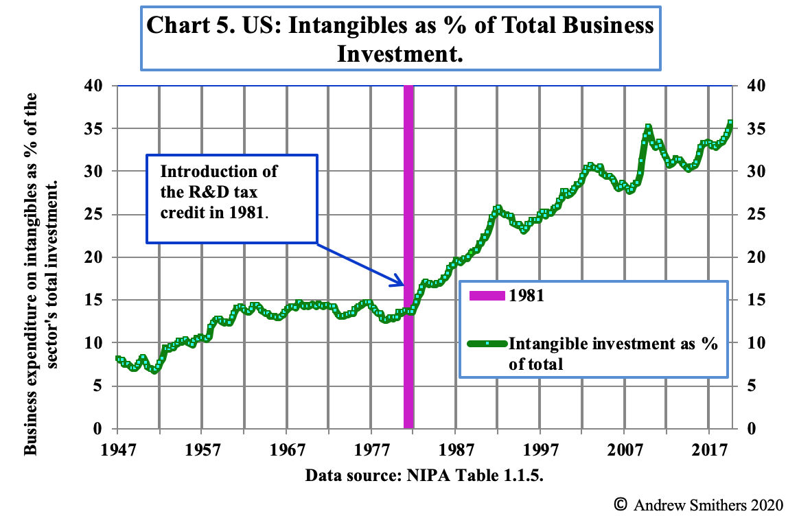
“There is a large tax credit in the US for R&D which was introduced in 1981. Chart 5 shows that business spending on IP averaged 12% of its total investment for 25 years before that and has since risen to over 36%. Over the same period total factor productivity (“TFP”), which measures the contribution to growth from improvements in technology, has seriously declined; however, this is measured.
We are therefore left with a choice between believing that companies have devoted more and more resources to R&D over the past 32 years for increasingly lower returns or that the rise in the amount attributed to R&D investment in the national accounts does not represent the extent to which expenditure on research has actually increased, but a renaming of spending. Anecdotal evidence points to companies reducing their tax, without any real increase in expenditure on IP, by categorising an increasing part of the salaries and other costs of employees, which were previously treated as general expenditure, as investment in R&D. There is therefore a strong possibility that investment in IP is mismeasured. The tax credit encourages companies to redefine expenditure which was previously allocated to general management to R&D and if this is done and accepted by the tax authorities and the national accountants as representing a true rise in such expenditure, the data will be distorted.”
(f) Professor Taylor queries whether net profit margins are mean reverting and asks for “more thorough statistical analysis.” This is not directly relevant to whether profit margins should be measured gross or net, but is set out below in James Mitchell’s comments on the statistics, which show that there is a case for the stationarity of net margins in accordance with the Cobb-Douglas production function. The longer the data series are the stronger the conclusions that can be drawn from them and time will therefore tend to confirm or raise doubt about the mean reversion of the series.
Statistical comment by Professor James Mitchell
I have run the profit share series (so rows 73, 80 and 87 of the xls file) using the full-sample (data from 1929-2019) through some standard and modified unit root or Augmented Dickey-Fuller (ADF) tests.[2] Results are computed using Stata, a commonly used software package.
The results, as is common, depend on the lag order chosen in the underlying autoregressive (AR) model used to mop up the serial correlation in the profit share series. Recall the null hypothesis in all these tests is of nonstationarity: so larger test statistics (in absolute value) make it more likely that we can reject the null. I have also implemented all these ADF tests including a constant but excluding a linear trend: so the alternative hypothesis is of stationarity (with no linear trend). This specification choice, at least, doesn’t appear to affect results.
In short, if you select a short lag order (so assume the first difference of the profit share, say, is best modelled just in terms of its value just last year: an AR of lag order 1) then one does convincingly reject the null of a unit root: the profit share is indeed mean reverting (p-values of 0.00). But as we increase the lag order, the evidence for rejection declines. So, by the time you get to including 12 lags (quite a lot for an annual series, it has to be said) you no longer reject nonstationary.
Please see the cited Word file, with the key results in red. These tables of results simply show the unit root tests and the underlying estimated coefficients and t-values on the lagged values in these different AR models for each of the 3 profit share series.
This sensitivity to the lag order of course raises the question, what do the data tell us is the preferred lag order?
To help get at this, and given the ADF test is well known to have low power (to detect mean reversion) in small samples, I also ran the data through a popular (more powerful) test,[3] which also selects (according to the data) the preferred lag order. Using this test and focusing on the lag order selected by the so-called Ng-Perron test (highlighted red in the attached), we see that these higher order lags are “liked” by the data. Hence the preferred (“optimal”) lag selected is pretty high (7); and consistent with the standard ADF tests (if we include more lags) for these variants of the Elliott et al. test nonstationarity cannot be rejected. But, if we use a different statistical criterion to select the preferred lag order (as you can see, Stata by default returns three), such as the Schwarz Criterion (denoted SC), then a lag order of 1 is selected: and one would again reject nonstationarity.
In summary, as is common, the data tell different stories depending on how you use them. As ever, in the presence of this statistical “uncertainty”, we should perhaps revert to our economic judgement to discriminate between the different tests. Here I believe there is a strong argument in favour of stationarity (mean reversion).
11th September, 2020
[1] I quote from The Debate over the Depreciation of Intangible Capital by Andrew Smithers World Economics Vol. 21 • No. 1 • January–March 2020
[2] The data series and the statistical tests are available on http://smithers.co.uk/download.php?file=900
[3] See https://www.stata.com/manuals1…. Elliott, G. R., T. J. Rothenberg, and J. H. Stock (1996). “Efficient tests for an autoregressive unit root”. Econometrica 64: 813–836.