How models treat innovation may be just as important as their assumptions about climate damages
Continued global warming will accelerate the damages and risks of climate change. Agreement on the need to avoid ‘dangerous interference’ in the climate system led to the goal of the Paris Agreement, to keep global temperature increases to the range 1.5-2.0 degrees Centigrade. This would mean rapidly reversing the historic trend of growing CO2 emissions, reducing towards ‘net zero’ within a few decades.
Whilst scientists have highlighted the climate risks, many economists have stressed the apparent costs of deep emission reductions, and debated the ‘optimal’ level of effort that would be justified on cost-benefit grounds. Many of the resulting models have suggested that a gradual increase in emissions abatement, deferring deep cuts for decades, would be optimal - even if that results in significantly higher temperatures. The most famous example is the DICE model pioneered by Professor William Nordhaus, one of a now large family of ‘Integrated Assessment Models’ (IAMs).
Criticism of such IAMs has focused almost entirely on how they cost climate damage and risks. In this paper we argue that something else in these models deserves just as much scrutiny - namely, how they represent technology, and specifically, the innovation and economic transformation processes that are clearly necessary (and ultimately, appear implicitly in almost any model).
In our new paper we argue that economists need to acknowledge dynamic realism – the role of inertia, induced innovation, and path dependence in our energy and related systems. In our paper, we illustrate the problem – and propose a solution - using the famous DICE model.
Consider the cost function for CO2 abatement in the DICE model, which represents the cost of cutting emissions at time t, relative to a ‘reference’ projection:
C(t) = [C0(t) x s(t) x μ(t)2.6 (eq. 1)
Here, C(t) is the cost of CO2 reduction as a fraction of GDP at time t, and µ is the fraction of the emissions that are abated, i.e. µ=0 in the absence of any policy and µ=1 in case of zero emissions. The exponent 2.6 means that abatement becomes increasingly (and non-linearly) expensive, the deeper the cutback. C0 and s are both scaling factors which decline over time at preset rates (see our paper, note 2).
Yet, there is something profoundly odd about this. The abatement cost at time t in such a model does not depend at all on abatement beforehand. Deep emission cuts in 2050 are equally expensive regardless of whether any efforts have been made up to 2045. Thus, the model assumes temporal independence.
This is clearly unrealistic. Consider the following.
First, energy infrastructure has a lifetime of several decades. Eq. 1 basically assumes that the price of achieving deep emission cuts in 2050 is wholly unaffected by whether or not we have previously deployed any renewable energy, efficient buildings, or electric vehicles and infrastructure; whether factories are in place to produce these; or how many recently-built coal plants will have to be abruptly dismantled before the end of their lifetime.
Obviously in reality there is inertia in the energy system: fast changes are more difficult and more expensive than smoother transitions. If we replace coal plants by renewables over thirty years, rather than in one year, we can gradually replace the oldest, most obsolete coal plants by wind farms, and forestall new ones, thereby minimising sunk capital. In addition, this lowers the peak rate at which we have to install low carbon systems, so we can achieve the same goal with fewer construction firms or factories. With its standard values, DICE takes 80 year to halve global emissions, then just 10 years to halve them again.
Moreover, previous abatement not only adds to the stock of green infrastructure, but also reduces the price of new installations as the industry builds up experience and supply chains over time. The more wind or solar plants installed, the better we get at building them, and the lower the costs become. Over the last 10 years, the cost of solar energy has dropped by a factor of 5. Across rapidly growing areas of the world, it has become the cheapest way of generating electricity. The cost of wind energy has also fallen, dramatically so for offshore wind. Not by some external magic, or some breakthrough innovation in labs, but because some countries deployed these at scale, giving producers the opportunity to learn, build up supply chains, and exploit economics of scale. The initial costs were large, but they proved to be transitional, because they induced innovation in technologies and industrial capabilities.
The same underlying characteristic, to a large degree, is true for infrastructure, whether high efficiency buildings or electric vehicle charging networks.
These two effects, induced innovation and inertia (including that associated with infrastructure), means that eq.1 cannot be correct. Abatement costs depend on previous effort, and may be largely transitional. It costs money to accumulate the knowledge needed to make a new technology work efficiently, and to actually replace infrastructure, but once a transition is achieved, the new, green technology is not necessarily more expensive than its fossil fuel counterpart. But the faster the transition, the more the peak expenditure needed. And the longer one defers the effort, the faster it will eventually have to be.
Economists have of course tried developing models with characteristics like this, but they tend to be very complex, and no IAM in widespread use does so. We suggest a far simpler way to explore the implications of dynamic realism. In our paper we show, step-by-step, the logic of adding a second term to eq.1 to represent inertia, and which can then be most usefully transformed to:

Here, p refers to the pliability of the emitting system and determines the extent to which costs are transitional or enduring and ![]()
![]() is the rate of abatement at time t. If p=0, there are no transitional costs, and abatement costs are entirely rigid – impervious to earlier abatement-related investment. This is the classical case represented by DICE. In contrast, if p=1, then the costs are purely transitional: they only depend on the rate of change of the abatement – the increase in abatement within a given year. K is a normalisation factor (which we show relates to the characteristic timescale of system response).
is the rate of abatement at time t. If p=0, there are no transitional costs, and abatement costs are entirely rigid – impervious to earlier abatement-related investment. This is the classical case represented by DICE. In contrast, if p=1, then the costs are purely transitional: they only depend on the rate of change of the abatement – the increase in abatement within a given year. K is a normalisation factor (which we show relates to the characteristic timescale of system response).
To investigate the policy implications, we implemented eq.2 into DICE and computed the optimal abatement trajectory for p=0, p=0.5 and p=1. The results are displayed in fig. 1.
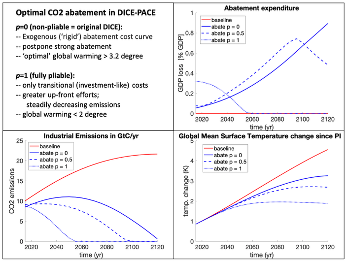
Optimal abatement in the DICE with Pliable Abatement Cost Element (DICE-PACE) model, for an (arguably, optimistic) characteristic transition time (see paper) of 20 years. The red line represents a baseline scenario with zero abatement (no climate policy), the blue lines represent the optimal policy results for p=0 (original DICE model), p=0.5 and p=1 (only transitional costs). The bottom left plot shows CO2 emissions in gigaton of carbon; the top right the cost paid for abatement (as percentage of GDP); and the bottom right the global mean temperature. Note that the mild damage function of the original DICE model has been used throughout.
For p=0, abatement starts very slowly, mostly because the model has quite a strong GDP growth and tends to postpone abatement “until the world is richer, and abatement is cheaper”. This is the classical behaviour of DICE and similar models.
But if abatement costs are purely transitional (p=1), then the optimal policy is a prompt start to bigger, but steady, emission reduction, driven by higher expenditure in the first 25 years. The reason is that in the p=1 case, every dollar spent for abatement is truly an investment for the future: any windmill or other low carbon infrastructure built today will continue to save CO2 in the future, and contributes to learning. Once the transition is achieved, the cost of staying at low or zero emissions drops to zero. This contrasts sharply with the opposite extreme of a totally rigid system (p=0) where abatement in one period brings no future emission benefits.
Readers might initially consider a case with p => 1 to be absurd. It indeed suggests that the costs of abatement are all transitional, and that in the long run, a low carbon energy system may be no more costly than a high carbon system. Yet there is increasing evidence, for that is what seems to be happening in electricity, and now seems entirely possible in road transport. Solar and wind energy are becoming cost competitive as they are deployed more widely, and storage (batteries) and other and system management options are rapidly becoming cheaper as well. Many processes that are currently driven by fossil fuels could be powered by cheap electricity. Electric cars, for example, are set to become cost competitive within a few years.
Indeed, there seems no fundamental physical reason to assume for the majority of energy uses that extracting carbon out of the ground, transporting, and processing it, and cleaning up its environmental impacts, is inherently cheaper than extracting energy locally from the sun and winds. Nor indeed to assume that complex combustion engines make for cheaper transport than the much simpler electric drive trains. The big question is whether we should expect the needed innovation to occur in the laboratory, or on the industrial field of deployment and scale economies. Our study presents a range of evidence pointing to the crucial role of the latter, which points to the technical pliability of energy systems.
Our intent, however, is simply to show how much this largely neglected aspect of IAM modelling matters. Beyond the near-term behaviour, it also follows - not surprisingly – that total emissions and thus global mean temperature are lower for a pliable system (p=>1) than for a rigid one (p=0). In fact, for p=1, the optimal warming stays below 2 degrees - despite the very mild assumptions in DICE about how damaging climate change will be.
We contend that these issues of dynamic realism are in fact far more tractable, more amenable to evidence, and even more relevant to practical policy than debates about costing climate damages, risks and long-term discounting. Our results show that how models treat innovation, in particular, may be just as important as their assumptions about climate damages.
It is time for economic modellers to move beyond the indefensible assumption of temporal independence. Incorporating the dynamic realities of energy and related systems is of fundamental importance to tackling climate change, and economics needs to rise to that challenge.