As so often in recent decades, developments in the US economy are puzzling the majority of economists and defying their predictions. The slow recovery that has followed the great crisis of 2008 has sent the unemployment rate, that had risen to 10 percent in 2009, down to levels (3.7 percent in August) paralleled only in the booming economy of the late 1960s. This steep and seemingly interminable reduction in unemployment, accompanied by a general improvement in all other labor market indicators, has raised anxieties among economists and policy advisers about the supposed inflationary risks that the American economy might face, even as world stock markets shake from the specter of trade wars and fears of a possible future recession begin to emerge.
Fighting inflation has for decades obsessed central banks and standard economic theory takes as a fact that unemployment below a certain threshold inevitably produces inflation, or, more precisely, accelerating inflation (as famously maintained by Friedman, 1968). This preoccupation had no small part in the U.S. Federal Reserve’s tightening of monetary policy from December 2015 on. The subsequent interest rate hikes, spreading over three years, amount to a cumulative increase of 2.5 percentage points. However, to the general amazement of the profession, not only has this tightening failed to check the fall in unemployment, which has instead continued up to the current historically low levels, but the latter has failed to produce the feared explosion in inflation. Money wages only in recent months have shown some tendency to a more sustained increase than in the past. According to the data released in September by the US Bureau of Labor Statistics, while job creation remains rather strong, [1] money wages increased at an annualized rate of about 3 percent. The fact that inflation has failed to materialize is reflected in falling long-term interest rates, also affected by expectations of slower growth. Urged on by critics, including President Donald Trump, the Fed has felt obliged to react by cutting rates by 25 basis points in late July, in what some regard as a belated and perhaps too timid move.
By the numbers, accordingly, there is no evidence that the US economy has crossed any ‘inflation threshold,’ despite the continuing (if slowing) growth and the very low unemployment rates. In mainstream economic theory, the inflation threshold is identified with the level of activity corresponding to the natural rate of unemployment (or NAIRU), the particular rate of unemployment that supposedly represents equilibrium in the labor market, thus being consistent with an absence of either inflationary or deflationary pressures. Strong as the theoretical belief is that a natural rate exists, over time economists and policy professionals have in practice encountered significant difficulties in giving it any precise empirical content. To cite just one example, the Congressional Budget Office of the United States currently estimates the natural rate to be 4.6 percent, which implies that actual output has been above potential since the second quarter of 2018 (see CBO, August 2019).
But this just points up the flimsiness of the whole approach. The problem is not simply that staying beyond the inflation threshold for five quarters in a row has failed to produce the feared inflationary consequences. There is also the now familiar problem of the moving target: In January 2015, the CBO projected a natural rate of 5.4 for 2015 and 5.3 for 2018. In January 2012, it had projected a 5.5-5.8 natural rate for 2015 and 5.5 for 2018. Not to speak of the late 1970s and early 1980s, when the natural rate was estimated to be way above 6 percent. These swings are nothing compared with the dizzying revisions that have affected the European Commission’s estimates of the analogous notion of NAWRU (non-accelerating-wage rate of unemployment) for some European countries. Spain’s NAWRU, for example, was estimated at about 20 percent in 2013; while the current estimate sets it at 14.9 percent for 2019, and, interestingly, revises the estimate for 2013 to 17.7 percent.
It is always possible to put forward rational sounding explanations of these changes, in light of better data, or more careful retrospective consideration of such factors as the age composition of the labor force, changes in participation in different population groups, and the like. But the feeling is inescapable that the revisions are obliged by the vagaries of the actual rate of unemployment, and the need for the theoretical notion of ‘natural rate’ not to lie too far apart from actual unemployment for too long a period. In a recent INET paper, we addressed these issues, not only showing how flawed the notion of natural rate of unemployment – and the potential output calculated on that basis – may be, both theoretically and empirically; but also proposing alternative calculations of potential output, entirely free from the notion.
By starting from a demand-led growth perspective, and rescuing A.M. Okun’s (1962) original method for estimating, we maintain there that potential output should be defined and calculated as the best possible approximation to a traditional Keynesian notion of full-employment output, understood as a sort of ‘maximum’ attainable output in any given situation. Obviously, such a maximum is not a true “maximum” in strictly technical terms. Like Okun’s original method, our method implies identifying an exogenously given ‘target’ rate of unemployment corresponding to a conventional measure of full employment (which takes into account, for example, the irreducible unemployment resulting from job changes, seasonality in some occupations and the like). By setting two conventional target rates at 4 and 3.4 percent respectively, in the paper we reconstruct, on that basis, two estimated potential output series for the US economy for the 1959-2018 period. Both yield a different account of the long-term evolution of potential output and the output gaps by comparison to standard estimates.
If the picture of the US economy in mid-2019, however, is particularly puzzling for standard economic theory, it also raises questions for such an alternative standpoint. With current unemployment so low, how close is the economy to ‘full employment’ proper? Is there any way of correctly gauging, in general, how much unemployment there still is at “full employment”? Perhaps more importantly, given that fears of recession or hopes for a “Green New Deal” bring about demands for stimulus, does the current state of the American labor market imply that the space for further expansion of demand and production is entirely exhausted? If instead there are margins, how big they are and how may they be quantified? Finally, since in Keynes’s analysis full employment proper was identified with the inflation threshold, should we not be witnessing a more sustained increase in wages and prices, independently of any belief in the untenable notion of the natural rate of unemployment?
Starting from the analytical framework proposed in our earlier paper, we will try here to address these questions.
Okun’s law and potential output
Following Okun’s (1962) original method, in our paper we rely on Okun’s law for calculating potential output. As is known, this is an empirical regularity connecting changes in the rate of unemployment to the rate of growth of output. In the original formulation of the law, Okun famously found evidence that any 1 percent change in real output would cause a change of about 0.3 percentage points in unemployment. That made it possible to calculate the change in output needed to bring unemployment to the desired value, and thus to indirectly reconstruct in this way a time series of potential output. As we note in the paper, in the light of the conceptual and practical difficulties with the notion of the ‘natural’ rate of unemployment and the empirical irregularity of the inflation-unemployment relationship, a major merit of Okun’s procedure lies with the fact that it refrains entirely from relying on either the natural rate concept (or any attempt to define an ‘equilibrium’ rate of unemployment) and from the use of inflation data in potential output estimation.
The possibility of calculating a meaningful measure of potential output through Okun’s procedure rests on the validity of the following propositions: a) the unemployment rate is a good indicator of labor underutilization; b) labor underutilization is, in any given situation, a good indicator of the general underutilization of resources; c) Okun’s law is reasonably regular. As regards this latter point we found that in general the fit of the relation is surprisingly good over quite long periods, especially when allowing the Okun coefficient to have different values for different ranges of the unemployment rate (see the paper for details). It has to be noted, however, that not only did we detect a structural break in the relationship in 2009, but also that the fit of the relation seems to be slightly less good in the recent years. Read together with the data pointing to a lower participation in the labor market than in previous phases of low unemployment, this could be interpreted – we surmised in the paper, without entering into details – as a symptom that the unemployment rate has ceased to be, in the recent phase, a sufficiently good indicator of labor underutilization.
Alternative indicators of labor underutilization: U-6
As noted above, despite the exceptionally low unemployment rate, the picture the American economy offers is quite mixed. Apart from the above-mentioned data on wages, other labor-market indicators do not seem to be at peak values. According to the BLS data referring to August, the labor force participation rate still lingers around 63 percent, well below the 66 percent rate prior to the Great Recession (see Figure 1). The long-term unemployed (those who have been unemployed for 27 weeks or more) are now about 1.2 millions, back to the level of 2007, but still much above the level of the previous peaks in activity (in 1999-2000, for example, they were half than that, not only in absolute terms but also as a percentage of the labor force).
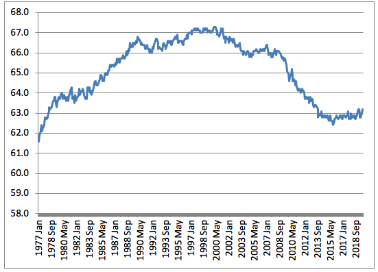
Figure 1. Labor force participation. USA, seasonally adjusted monthly data (1977Jan-2019Aug) Source: Current Population Survey, US Bureau of Labor Statistics
To determine whether there is hidden unemployment, we may in the first place refer to the broadest indicator of labor underutilization provided by the BLS, the rate U-6. The latter is built by adding to unemployed proper (those who searched actively for work in the last month prior to the survey without finding it) those that, although without actively searching for a job, would however be prepared to work were some job available (so-called ‘marginally attached workers’), and also those part-time workers that work less hours than desired because of the unavailability of full-time jobs. This sum is then expressed as a ratio to the labor force augmented by marginally attached workers. Similarly to the official unemployment rate, the rate U-6 rose to historically high values during the Great Recession (17 percent in 2009Q4), decreasing steadily since then. At 7.2 in 2019Q2,[2] U-6 is currently almost at the minimum level recorded in its time series (6.9 in 2000Q4; but notice that data for U-6 are reported only since 1994). Another indicator that gives an idea of how hidden unemployment relates to the ‘open’ one is the difference between U-6 and the official unemployment rate (also called U-3). This difference greatly increased during the crisis and is now back to pre-crisis levels; however, at 3.5 percent percentage points in August, it is still slightly above its minimum (3.0) reached at various quarters in the peak of activity of 1999-2000.
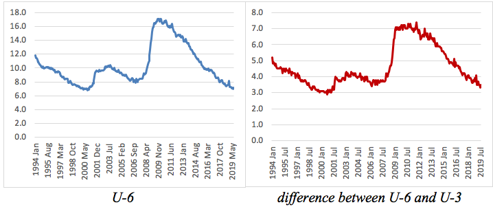
Figure 2. U-6 and difference between U-6 and U-3. USA, seasonally adjusted monthly data (1994Jan-2019Aug) Source: Current Population Survey, US Bureau of Labor Statistics
Even if the picture offered by U-6 differs only marginally from that offered by U-3, it is worth examining how Okun’s law relates to this different ‘broader’ unemployment rate. To do this we regress the first difference of U-6 on the rate of growth of output using quarterly data on the 1994Q1-2019Q2 period. We find that this variant of Okun’s law works as well as the original one.[3] Similar to what we found in the paper with the U-3 rate of unemployment, the best model is one that allows for different values of the Okun coefficient according to the low, medium or high value of the ‘broad’ rate of unemployment. (The intuition is that unemployment reacts more to output growth when unemployment itself is high, while for very low rates of unemployment much of output growth is accommodated by changes in productivity due to more intensive use of labor. See the paper for details). The table reports the resulting values of the Okun coefficient.[4]
Table 1. The Okun coefficient with the ‘broad’ unemployment rate U-6
| Different ranges of U-6 | Cumulated Okun coefficient (contemporaneous plus lagged effects) |
| Low range (𝑢6𝑡 < 8.9) | -0.39 |
| Medium range (8.9 ≤ 𝑢6𝑡 ≤ 10.3) | -0.74 |
| High range (𝑢6𝑡 > 10.3) | -0.99 |
Okun’s law seems thus to be quite a robust relation, which holds also with alternative indicators of labor underutilization. We can now use our result to produce a different measure of potential output, based on U-6 instead than U-3, to assess the current measure of the US output gap and compare it with that obtained by using U-3.
An important issue is which level of U-6 to select as a desirable target. That is also affected by the chosen target level of U-3, the official unemployment rate. The lowest target of U-3 we chose in the paper, i.e. 3.4 percent, was the minimum recorded level of unemployment in the 1959-2018 period. In principle, there are no obstacles to targeting a still lower level, especially since the 3.6 unemployment of some recent months has failed to produce appreciable inflationary pressures. It is also difficult to say how high ‘irreducible’ unemployment is, and thus which exact value of the rate of unemployment corresponds to full employment. [5] In order not to set too ambitious a target, we calculate the gaps with two different U-3 target rates, 3.4 and 3.2 percent (although the latter possibly represents a conservative measure of full employment proper).
As regards U-6, the historical record (from 1994Q1 on) gives 6.9 percent as the lowest observed value (in 2000Q4). This is a possible target. Even more than in the U-3 case, there is however neither an objective nor a conventional criterion by which to determine the level of U-6 that is socially desirable and may be taken as approximately corresponding to full employment. One possibility is to rely on the difference between U-6 and U-3 described above, and take as a criterion that this should be minimized (as happens historically in phases of high activity). So we determine also an ‘ambitious’ U-6 objective by adding this minimum difference to our lowest U-3 target. In sum, we calculate potential output and output gaps first in terms of U-3, targeting either 3.4 or 3.2 percent, and then in terms of U-6, targeting either 6.9 or 6.2 percent. The resulting gaps are shown in the table below (for calculation of current potential output in terms of U-3 we rely on the coefficients estimated in our paper).
Table 2. Possible alternative measures of the output gap at 2019Q2
|
|
| U-3 | U-6 | ||
| Target |
| 3.4 | 3.2 | 6.9 |
6.2
|
| Gap at 2019Q2 in terms of the target |
| 0.2 | 0.4 | 0.3 | 1.0 |
| Output gap as % of actual output |
| 0.7 |
1.4
| 0.8 | 2.6 |
| Output gap in current billion dollars |
| 147 | 295 | 164 |
546 |
Although estimates of Okun’s law and the calculation of output gaps involve real output at chained prices, in the last row of the table we translate the measure so obtained into current dollars to give an immediate idea of the size of the gaps in terms of yearly GDP.
The different hypotheses of course give different output gaps: these derive from the conventional nature of the full employment target and the possibility of defining it in different ways. On the whole, however, the estimated gaps are quite limited in size. We should either conclude that there is not much space left for further expansion – which however is contradicted by some of the evidence we quoted in the beginning – or that labor underutilization has ceased to be, recently, a reliable indicator of capacity and resource underutilization.
The latter might indeed be the case. The non-exceptional growth in GDP in recent years seems actually to have been realized by greatly increasing the use of the labor input, which implies that margins of further expansion should probably be sought for in a more efficient use of labor rather than in further increases in employment. Before exploring this route, however, it is worth pausing a moment to wonder whether the U-6 indicator is actually appropriate for correctly estimating the extent of labor underutilization. The very low values recently reached by U-6 do not in fact square with the data above on labor force participation. Although U-3 and U-6 are at historically low levels, the participation rate is still much below its peak values, and it is doubtful that this can be entirely explained by changes in the age composition of population. We may note in fact, for example, that also in the 25-54 age range the participation rate, although recovering lately, is still below the 2007-8 value and much lower than its historical maximum value (reached in 1997 and 2000).
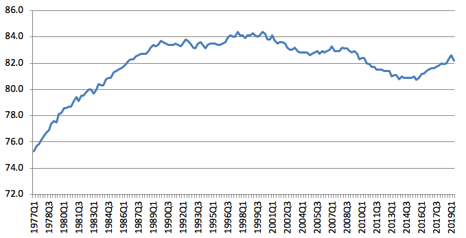
Figure 3: Labor force participation rate, 25-54 years. USA, quarterly data (1977Q1-2019Q2) Source: Current Population Survey, US Bureau of Labor Statistics
We thus explore the possibility that different indicators may better account for labor utilization.
Hours worked
The most reliable direct measure of labor input is the total amount of hours worked in the economy. The following figure shows the strong positive correlation between the rate of growth of total hours worked and the rate of growth of output, on US quarterly data over a long period (1959Q4-2019Q1).
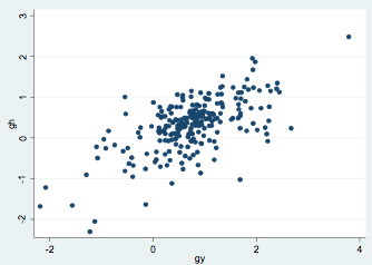
Figure 4. Scatter diagram: rate of growth of hours worked (gh )vs rate of growth of output (gy). USA, 1959Q4-2019Q1
The strength of the relation is confirmed by the good fit of the regression of hours growth on output growth – allowing for lags of the independent variable, we obtain a significant and fairly stable relationship with a single structural break in 1974Q4[6]. Obviously, this is not a one-to-one correlation, since increases in output are accommodated also by increases in productivity, along with changes in hours worked, and because the proportion between the two varies across sectors and productions.
To make intertemporal comparisons and assess the extent of labor utilization, we express total hours worked as a ratio of the working-age population. We do this to define a sort of ‘standardized’ indicator that is not influenced by the changing size of the economy.[7] The working age population may be defined, alternatively, either as the population between the ages of 16-64 or as the whole population of 16 years or more. Since there are many workers in the 65+ range and employment in this age range has been increasing steadily in the last couple of decades, the second definition looks more appropriate. However, given that there has been some change in the age composition of the population in favor of older cohorts, and since the latter on average work less or fewer hours, the indicator might be biased. So we opt for using both definitions, and build two different indicators, i.e. (annualized) hours worked divided by “prime working age” population (HPAP) and (annualized) hours worked divided by the population with 16 years or more (HPOP)
HPAP=(total hours worked)/(population 16-64)
HPOP=(total hours worked)/(population 16+)
The following graph depicts the evolution of the two indicators over time (1977Q1-2019Q2):
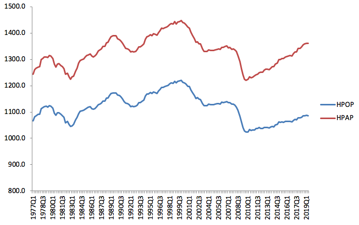
Figure 5. Annualized total hours worked divided by 16+ population (HPOP) and divided by 16-64 population (HPAP). USA; quarterly data (1977Q1-2019Q2) Source: our elaborations on data of the US Bureau of Labor Statistics
Table 3. Possible alternative measures of the output gap at 2019Q2
|
|
| U-3 | U-6 | HPAP | HPOP | ||
| Target |
| 3.4 | 3.2 | 6.9 | 6.2 | 1447 | 1221 |
| Current gap (at 2019Q2) in terms of the target |
| 0.2 | 0.4 | 0.3 | 1.0 | 85 | 136 |
| Output gap as % of actual output |
| 0.7 | 1.4 | 0.8 | 2.6 | 8.6 | 16.3 |
| Output gap in current billion dollars |
| 147 | 295 | 164 | 546 | 1843 | 3469 |
The distance is striking between the current level of the indicators (in 2019Q2) and their peak values (recorded in 1999Q4 for both series), despite the growth of hours worked in recent years. The annualized hours worked divided by prime-age population (16-64, HPAP) are now 85 less then at 1999Q4, which amounts to a 6 percent gap. As regards the other indicator, i.e. the annualized hours worked divided by 16+ population (HPOP), the gap with respect to its own peak value is even bigger: 136 in absolute terms, amounting to a 11 percent gap.
It is thus apparent that the quantitative use of the labor input in the US economy is not currently at its maximum. Leaving aside for a moment the desirability of such a move (on which more below), we may calculate how big an increase in current output would be necessary in order to bring these two indicators to their historical maximum levels. In order to do so, we first regress each of the two indicators, separately, on the rate of growth of output.[8] Obtaining significant and stable relationships, we then use the estimated coefficients to calculate these two different measures of the output gap. We show the results in the following table, which also reports, for comparison, the output gaps previously obtained with the U-3 and U-6 indicators.
Table 3. Possible alternative measures of the output gap at 2019Q2
| U-3 | U-6 | HPAP | HPOP | ||||
| Target | 3.4 | 3.2 | 6.9 | 6.2 | 1447 | 1221 | |
| Current gap (at 2019Q2) in terms of the target | 0.2 | 0.4 | 0.3 | 1.0 | 85 | 136 | |
| Output gap as % of actual output | 0.7 | 1.4 | 0.8 | 2.6 | 8.6 | 16.3 | |
| Output gap in current billion dollars | 147 | 295 | 164 | 546 | 1843 | 3469 | |
As is apparent, the calculations based on hours worked instead of the two unemployment indicators give a quite different picture of the current situation of the US economy. When measuring the labor input on the basis of the rate of unemployment, however broadly calculated, we should conclude that the US economy is currently performing very well, having reduced to historically low levels the number of those who want a job and are not able to find it. When the current situation is judged from the point of view of hours worked, instead, the extent of the current use of the labor input is considerably less impressive, and a sizeable gap appears with respect to other historical peaks of activity. If the American economy should now start growing more or more quickly, contrary to the current slowing down in the rate of growth, for example as an effect of a new stimulus package, the implication is that there would still be labor reserves to draw on.
Margins for expansion in the labor input
One may wonder where to find, in the current state of the US economy, such reserves of unused labor. The answer is not univocal, of course, because much depends on the nature of the supposed increase in demand, the sectors it stimulates and the types of jobs it creates. Some considerations at a general macroeconomic level are, however, possible. In the first place, the fact that the official (U-3) unemployment rate is now very low in historical comparison does not mean that it cannot fall more. Apart from the fact that 3.7 is not necessarily the lowest possible rate of unemployment, simple observation shows that for some groups and categories of the population average unemployment rates are much higher than for other groups. The average rate of unemployment in the black population, for example, is still 5.5 percent, well above the average rate. That historically the gap between black and white unemployment rates has always been there, at least since the 1960s, does not imply that it cannot be reduced further (a trend toward reduction is already visible lately). It must be noted that the declining black-white gap in unemployment rates goes together with a higher volatility of black unemployment, i.e. a greater reactivity of the latter to the economic cycle.[9] If this implies, on the one hand, that black employment is characterized by a greater share of temporary jobs and unstable occupations, it also points to the fact that sustained economic expansion may have a stronger effect in reducing black unemployment.
However, in the second place, it is clear that the different stories told by the indicators of unemployment (however broadly measured) and the count of hours worked are mainly explained by the data on labor force participation. As noted above, participation is markedly lower than in previous peaks of activity, not only if measured for the whole population of 16 years or more, but also if referring only to the central age classes (25-54). Broad indicators of participation, such as the labor force augmented with the so-called ‘marginally attached workers’, give similar pictures.
The gaps revealed by the above-described indicators of hours worked divided by working age population with respect to their peaks are thus mainly explained by the reduction in the share of the population employed, rather than by the decrease in hours worked per worker, which in the USA has been less intense, on average, than in the other OECD countries.
Participation tends normally to rise in expansions, as an effect of the increase in opportunities to work. The failure of the long expansion of the 2010s to raise participation back to the previous peak levels may thus be interpreted as a sign that further expansion has still wide potential reserves to draw on. It may also be a sign of the current weakness of economic incentives, in terms of the quality of the job opportunities that the US economy has been producing in the last years.
The argument should be mentioned that labor reserves are actually less wide than might appear, due to some structural change in the American population that has supposedly made greater shares of it ‘non employable’. The historical rise in the numbers of recipients of disability benefits, the alarm about the great numbers involved in opioid addiction, or the enormous growth in the prison and jail population (from half a million in 1980 to more than two millions now) are often quoted, in this respect, as causes for that sort of structural changes. Each of these issues would require careful analysis, and we are not going here into details. We may note, however, that such phenomena might also be interpreted, at least in part, as undesirable effects of the highly unequal character of the American economic growth of the last decades, which has increasingly penalized large sections of the population in terms of both quality of work and wages and more general living conditions. Without assuming that any simple and straightforward relationship may be established between social and economic magnitudes,[10] we may at least question the direction of causation implied in the usual account and suppose that the increasing trend in these phenomena of social distress might well be corrected and reverted, if this should become a policy objective. Moreover, as a rule, the increase in the creation of jobs opportunities implies that employment grows even in those categories of the population usually regarded as little employable or non-employable at all.[11]
Take the case of disability, for example. The number of applications for disability benefits has increased enormously starting from the early 1980s. According to the data of the Social Security Administration, benefit recipients, who amounted to less than two millions in 1970, are now more than 10 millions. While the main cause behind this rise in numbers lies with the institutional changes that in the 1980s made requirements for application less stringent, according to some studies there is also evidence that disability benefits have been used as substitutes for labor income, especially by some categories of low-skilled job losers, due to the growing ratio between the size of the benefit and the average wage of low skilled jobs, particularly in some areas of the country. Accordingly, disability numbers would also include a part of disguised unemployment. As evidence of a certain elasticity in at least a part of the pool of disabled workers to the change of economic conditions, we may note that recently, since 2015, the number of applications for disability benefits has started to decrease, apparently in connection with the uninterrupted creation of new jobs.
The ceiling that moves
We may sum up our findings so far: notwithstanding the very low rates of unemployment (both the official and the broad ones), it is very doubtful, in our view, that the US economy has reached a condition of true full employment, both because data for wages and inflation do not point to an overheated economy and because alternative indicators, as those based on participation or total hours worked, tell a different story. To measure precisely how much expansion could still be obtained at current techniques and current capacity, simply by increasing utilization of labor, is however quite a complex matter. As shown above, since the choice of the target is necessarily conventional, different indicators may be targeted, and at different levels: the output gap will have very different sizes accordingly (see tables 2 and 3 above). Our procedure, thus, though generally indicating that there are still margins for output expansion, does not allow us to quantify them through a single figure. This quantitative uncertainty we regard as inevitable, being associated with the necessarily conventional nature of the very notion of full employment.
Let us however assume, for a moment, contrary to what maintained until now, that it is currently either impossible or undesirable to further expand the quantitative use of labor. Let us suppose, for example, that the previous peak in hours worked was associated with excessive workloads and that a move towards a general reduction in hours is regarded as socially desirable.[12] Also in such a case, however, there would be no reasons to conclude that the margins for expansion are exhausted. There is in fact one dimension of labor underutilization that none of the indicators we have been using up to now is able to capture, and this has to do with employment in low-productivity occupations. The recent decades have been characterized by an increasing weight in the US economy of low-productivity (and low-wage) jobs, in a trend (common to most advanced economies) towards increasing polarization both in the labor market and in society at large (Storm 2017; Taylor and Ömer 2018). This reflects, as shown by table 4, in a slow growth of the average labor productivity of the whole economy, if compared to other expansion phases in the past.
Table 4. Average rate of growth of hourly labour productivity - total economy; USA, expansion phases of business cycles
| Hourly productivity | 1982q4-1990q3 | 1991q1-2001q1 | 2001q4-2007q4 | 2009q2-2019q2 |
| quarterly growth | 0,4 | 0,5 | 0,5 | 0,2 |
| annualized growth | 1,7 | 1,9 | 2,1 | 0,9 |
Should the economy be stimulated by a sustained increase in demand, accommodating increases in production could be obtained by increasing the efficiency in the use of labor through transfer of labor from low-productivity to high-productivity sectors and occupations, as has happened historically in all phases of sustained growth. This brings us to some wider considerations about the possible effects of aggregate demand in the economy.
All of our previous argument, as well as the updated Okun method for potential output estimation that we proposed in our earlier paper, are based on the attempt to quantify, in each period, the margins for output expansion that would arise from a fuller use of labor, given capacity and resources. As we tried to show in the paper, however, there is another powerful kind of effect that high levels of aggregate demand has on growth, and this consists in its capability to affect the very creation (or destruction) of resources. By inducing faster growth of capacity and productivity, high demand growth, while allowing the system to exploit existing production margins, at the same time widens those very margins by fostering more investment in physical capital and more rapid technical progress. That demand may have such powerful effects, a long-standing proposition of demand-led growth theory (Storm, 2019), is nowadays sometimes broached even in mainstream analyses, as they survey the disruptive effects that the Great Recession has had both on the level of activity and on the rate of growth.
The full-employment ceiling is thus not a fixed magnitude, independent of the difficulties of precisely quantifying it. It is rather a ceiling that moves over time. While strong current demand would create more space and allow for faster growth in subsequent periods, sluggish current demand slows down the creation of capacity, reducing the possibilities of future growth, including resources needed for “green growth.” A more accurate estimate of current margins for expansion would thus imply making some hypotheses on the possible effects of stronger demand on productivity growth (which may initially also be obtained through a more efficient use of inputs, at given techniques, and subsequently through an acceleration of technical change), and on its cumulative effect in the next few years.[13] If this adds further complications to the task of precisely quantifying the margins for expansion, it reinforces nonetheless the idea that such margins are anything but exhausted.
Where is the inflation threshold?
We may now go back to the last question we posed in the beginning, as regards both the failure of sustained inflation to materialize, notwithstanding the very low unemployment rates, and the possibility of identifying an inflation threshold, in our demand-led growth theoretical perspective. Standard theory has obvious difficulties here. In the last couple of decades, inflation has persisted at moderate or very low levels despite great changes in the rate of unemployment. The unemployment-inflation relationship has recently shown so flat a slope as to put into question the very existence of a significant (traditional) decreasing Phillips curve, let alone the possibility of identifying a natural rate of unemployment and the vertical Phillips curve (see for example Figure 6).
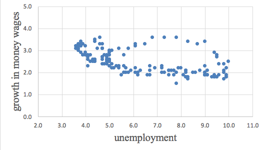
Figure 6. Unemployment vs growth in hourly money wages. USA, monthly data (12-month change); 2007Mar-2019Aug Source: our elaborations on data of the US Bureau of Labor Statistics
The history of the attempts to find empirical confirmations of the existence of the Phillips curve shows that generally the unemployment-inflation relationship is too irregular – both in the short and in the long period – to be a safe guide for policy (see our paper for details). Not only cannot inflation be seriously curbed by curtailing demand and employment, when cost-push factors are too strong, but it also does not necessarily explode at very low unemployment, when cost-push factors are very weak. Notwithstanding the theoretical dominance of the Phillips-curve for the last 60 years, and the consequent deeply-rooted belief that the level of activity and employment is the main determinant of inflation, cost-push factors are so relevant in practice that their role is generally recognized even in mainstream analysis. Recent trends in inflation, often puzzling for the mainstream account, are in fact often explained by stressing the increasing weight of global factors, such as trends in commodity prices, or exchange rates, or even referring to conflict over distribution – a fundamental determinant of inflation in heterodox approaches. Besides exposing the difficulties of mainstream theory, this constitutes in our view a more general warning against too mechanical reliance on the existence of a clear-cut relationship between the level of activity (or unemployment) and the dynamics of wages and prices.[14]
Our analysis also shows that to rely on a single indicator (the unemployment rate) to gauge labor underutilization and to determine whether or not an economy is at full employment may be, at least in some historical phases, grossly misleading. Other indicators show that the US economy is likely still below the full-employment ceiling and that the latter admits of different approximations.
What would happen if we tried to push the economy towards such a ceiling (however difficult may be to measure it)? Here we may note that full utilization of labor and capacity in the short run is by no means the ultimate barrier beyond which uncontrollable inflation necessarily explodes on a long-period basis. Apart from the effects of external and other cost-push factors, which as a rule are not strictly related to the level of activity, the reasons why inflation tends to accelerate when approaching ‘true’ full employment are generally of two kinds: the first associated with a faster growth of money wages thanks to the improved bargaining position of workers, the second with possible shortages in capacity (plants, qualified labor, intermediate goods, etc) leading to increasing costs. The first determinant of inflation is at the moment very weak in the American economy and will likely be so for some time in the future (Taylor, 2019). As regards shortages of capacity, they would likely start to appear in some specific sectors, which implies that a carefully guided expansionary policy could either target different sectors or specifically address such shortages (or both). But even if such short-period inflation barrier should materialize under stronger demand pressure, this could well be a short-period phenomenon, since over time capacity reacts to demand stimuli, new capacity is created and the inflation barrier is pushed further on.
What can be done
Thus the argument that there is no room, in the current state of the US economy, for fiscal expansion, is clearly pointless. Contrary to appearances based on the low unemployment rates, even from a quantitative point of view utilization of the labor input is now way below its maximum, despite the fact that ‘maximum’ has been defined in the limited sense of the historically recorded peaks of activity. Fiscal expansion is badly needed, as increasingly recognized in unsuspected quarters as the ineffectiveness of monetary policy in fostering growth and sustaining the dynamics of prices becomes more and more apparent. As maintained above, a determined policy of demand expansion is not only necessary for contrasting the possible looming recession, but is the essential precondition for stronger growth in the future, thanks to its powerful effects on the supply side.
However, if there is a fundamental conclusion that the current state of the American economy suggests, it is that the profoundly unequal character of the economic growth of the last decades not only cannot be endured much longer by large strata of the society, as the indicators of growing social distress mentioned earlier suggest. This is also undesirable from a strictly economic point of view. As noted above, the low level and the slow dynamics of wages in many sectors and occupations – a prominent feature of the current evolution of the US and many other economies – are strictly connected to the qualitative dimensions of labor underutilization, i.e. the disproportionate weight in the economy of low-productivity jobs and sectors on which we remarked above.
This means that the actual content of any intended stimulus package, the investments it produces, the beneficiaries it targets and the sectors it aims to foster, cannot be considered as secondary or irrelevant. The possibility for the US economy to expand in the short term and to achieve higher and healthy growth in the long term seems to be inextricably linked to the issue of income distribution.
References
Autor, D. H., Duggan, M. G. (2003), The rise in the disability rolls and the decline in unemployment. The Quarterly Journal of Economics, 118(1), 157-206.
Currie, J., Jin, J., Schnell, M. (2019), US Employment and Opioids: Is There a Connection?, Health and Labor Markets (pp. 253-280). Emerald.
Congressional Budget Office (2019), An Update to the Budget and Economic Outlook: 2019 to 2029, August.
Eisner, R. (1998). Investment, National Income and Economic Policy. Edward Elgar, United Kingdom
Fontanari, C., Palumbo, A., Salvatori, C. (2019), Potential Output in Theory and Practice: A Revision and Update of Okun’s Original Method. Institute for New Economic Thinking, Working Paper No. 93, available at https://www.ineteconomics.org/…
Forbes, K. J. (2019), Has globalization changed the inflation process? BIS Working Papers, No. 791.
Friedman, M. (1968), The Role of Monetary Policy. The American Economic Review, Vol. 58.
Ghertner, R., Groves, L. (2018), The opioid crisis and economic opportunity: geographic and economic trends. ASPE Research Brief, 1-22.
Okun, A. (1962), Potential GNP: Its measurement and significance, Proceedings of the American Statistical Association, Business and Economic Statistics Section, ASA, Washington, 98-104.
Storm, S. (2017), The New Normal: Demand, Secular Stagnation and the Vanishing Middle-Class. Institute for New Economic Thinking, Working Paper No. 55, available at https://www.ineteconomics.org/…
Storm, S. (2019), Summers and the Road to Damascus. Institute for New Economic Thinking Blog, available at https://www.ineteconomics.org/…
Summers, L. H., Stansbury, A. (2019), Whither Central Banking?, Project Syndicate, available at
https://www.project-syndicate….
Taylor, L., Ömer, Ö. (2018), Where Do Profits and Jobs Come From? Employment and Distribution in the US Economy. Institute for New Economic Thinking, Working Paper No. 55, available at https://www.ineteconomics.org/…
Taylor, L. (2019), Central Bankers, Inflation, and the Next Recession. Institute for New Economic Thinking Blog, available at https://www.ineteconomics.org/…
[1] A word of warning should be added. Data on job creation are provisional, and are usually revised months later. The Current Employment Statistics Preliminary Benchmark Announcement of August 21st has in fact indicated that, in the year ending in March 2019, job creation may have been overestimated by half a million. Final revisions will be available only in February 2020.
[2] Also in August 2019, according to the latest data release, U-6 is at 7.2 percent.
[3] We regress the first difference of U-6 on the rate of growth of output (contemporaneous and lagged up to two periods). Both dependent and independent variables are stationary. Since the disturbances are heteroskedastic and follow an AR(1) process, we estimate an ARMAX (1, 0) model with robust standard errors which includes two lags of the independent variable (the number of lags for both variables have been chosen through various information criteria). We take into account the presence of a structural break in 2011q1. According to the R-squared, our model predicts 77 percent of the variability of U-6. Further details are available on request.
[4] The limit values for the three ranges have been chosen on the criterion that each of the three ranges contains about a third of the observed values. Compared to our precedent estimation with U-3, results are qualitatively confirmed: signs of coefficients, significance of the three ranges of unemployment and their ordering are those expected.
[5] The literature of the last decades has given little or no attention to the question of the exact measurement of full employment, given the theoretical and practical dominance of the economics of the natural rate. In what represents one of the few exceptions, Robert Eisner (1998, p. 422) noted that the Humphrey–Hawkins Full Employment Act of 1978 was perfectly sensible in “setting a goal of 3 per cent ‘adult’ unemployment, corresponding to minimal friction and search unemployment, as the full employment target”.
[6] We regress the rate of growth of hours worked on the rate of growth of output (contemporaneous and lagged up to two periods). Both dependent and independent variables are stationary. The disturbances are homoskedastic and not serially correlated. We therefore estimate an OLS model which includes two lags of the independent variable, chosen by comparing different information criteria. We also take into account the presence of a structural break in 1974q4. According to the R-squared, our model predicts 58 percent of the variability of growth in hours worked. Further details are available on request.
[7] Our indicator is thus a sort of employment ratio, in which however employment is measured in terms of total hours worked (regardless of their distributions among the employed) instead of number of employed persons. The rationale for such a choice lies with the attempt to measure the total (standardized) labor input allowing also for possible changes in the number of hours worked per employed person, due to overtime, diffusion of part-time work and the like.
[8] We regress the first difference of each indicator on the rate of growth of output (contemporaneous and lagged up to two periods). Both dependent and independent variable are stationary. The disturbances follow an autoregressive process; therefore, we estimate an ARMAX (5, 0) model which includes the contemporaneous and lagged independent variable (only significant lagged terms are included according to the parsimony criterion). The selection of the best model and of the optimal number of lags for both variables have been made by comparing different information criteria. According to the R-squared, our model predicts 60 percent of the variability of HPOP and HPAP. Further details are available on request.
[9] Separate estimates of Okun’s law for black and white unemployment rates give a reactivity of unemployment changes to output changes that is almost double in the case of black unemployment (estimates have been run on quarterly data on the 1977q1-2019q2 period).
[10] In the case of opioids, for example, while some studies regard the abuse of opioids as a possible cause of slower growth through reduced participation, others on the contrary regard it as an effect of worsened economic conditions, and others doubt that any clear relationship may be established between trends of opioid abuse and economic indicators.
[11] A case in point is the recent tendency, on the part of employers, to relax education and experience requirements.
[12] Although we are not maintaining that such a more desirable social arrangement is what lies behind current data on hours worked, given the evidence discussed above.
[13] For example, an additional growth of productivity of 0.2 percentage points quarterly (thus replicating the growth in productivity recorded in the 1980s, which is by no means the highest historically) would imply, other things being equal, 4 additional percentage points in output growth in five years.
[14] It should be noted that NAIRU models (such as Carlin and Soskice, 1990), even if based on explicit recognition and modeling of conflict-based inflation, do produce standard results in terms to convergence to a unique equilibrium due to reliance on continuous univocal functions relating bargaining power to unemployment and standard adjustment mechanisms.